论文精读 · Block Sparse Attention with Log-Linear Complexity (PISA)

01 · Overview

速览

这篇论文要解决一个很具体、也很要命的问题:块稀疏注意力省下了注意力计算,却没省下"挑哪些块"的开销。传统做法(BSA)要给每个 query 对全部 $N/C$ 个键块打一遍分,于是选择阶段总开销是 $O(N^2/C)$——注意力本身降成线性了,选块却还是二次的,在长序列上直接成为新瓶颈。作者提出的 PISA 用"键的金字塔 + 由粗到细的逐层 Top-K"把这个阶段压到每个 query $O(\log N)$、整段序列 $O(N\log N)$。

核心机制

金字塔 Top-K 选择均值池化建 $O(\log N)$ 层键层级,从最粗层逐级展开、每层只对至多 $gK$ 个候选打分

打分函数

LogSumExp 块打分不是对子块均值求平均,而是在子块摘要上做 LSE,理论上更贴近真实块质量

复杂度

O(N log N) 预填充 / O(log N) 解码对比 BSA / NSA / MoBA / HiLS 的 $O(N^2)$ 与 $O(N)$

选择延迟

比 BSA 快 9.95×256K 长度预填充选块阶段;128K 为 5.31×,64K 为 2.86×

选择质量

Recall@8 90.95%同 query/key 下对比 BSA 的 85.91%(论文 Table 7)

长上下文

RULER 平均 62.802.67B、16K 上对比 BSA 的 54.99(论文 Table 3)

读数约定:本页全部数字以论文原文为准;凡由本页依据论文配置整理、归纳或换算的内容,均以「整理」「推算」显式标注,便于与论文口径区分。记号沿用论文:$N$ 为序列长度,$C$ 为块大小,$K$ 为保留块数,$g$ 为层级分支因子(论文取 $g=2$),$\ell$ 为层级编号($\ell=0$ 是原始键,$\ell=1$ 是叶块),$d$ 为头维度。论文未给出代码仓库地址。

三句话读完

问题。块稀疏注意力分两步:先为每个 query 挑 $K$ 个键块,再只在这些块上算注意力。第二步是线性的,但第一步要对全部 $N/C$ 个块打分,整体仍是 $O(N^2/C)$。序列越长,这个"选块"越像新的全注意力。

做法。把键逐级均值池化成一个由细到粗的金字塔($C$ 个一组、之后每 2 个一组),然后反过来从最粗层往下选:每层只对上一层保留下来的块的孩子打分,保留 Top-$K$,再展开到下一层,直到叶块。每层候选数被 $gK$ 卡住,层级数只有 $O(\log N)$,于是每个 query 的选择开销是 $O(\log N)$。打分的度量从"子块均值的平均"换成"子块摘要上的 LogSumExp",论文用 Jensen 不等式给出了它夹在「均值平均」与「父块真实 LSE」之间的论证。

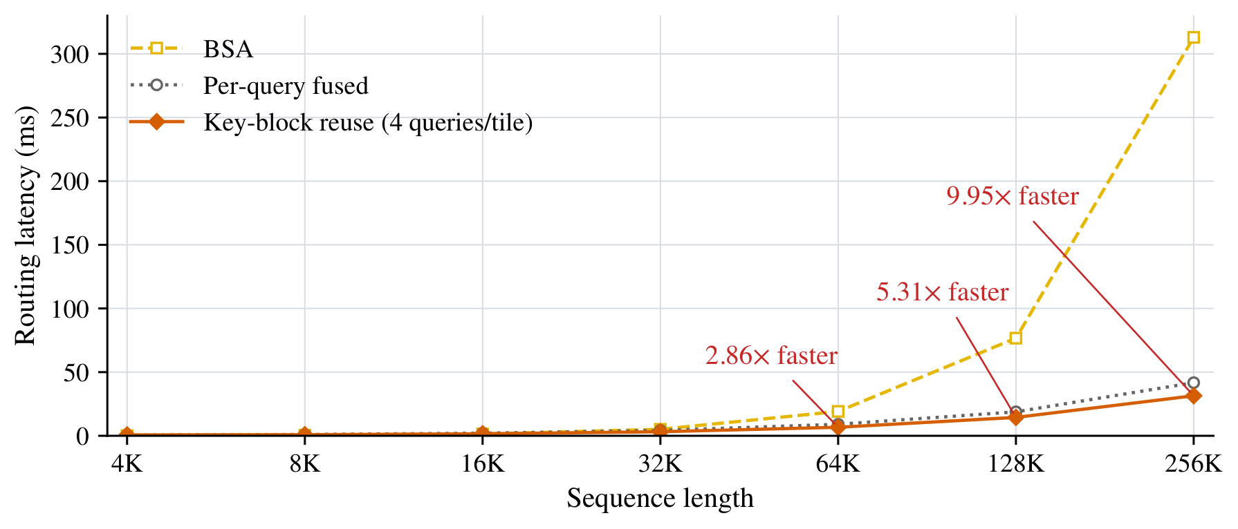
结果。418M / 1.47B / 2.67B 三个规模、100B token 预训练 + 10B token 16K 继续预训练下,语言建模损失与常识推理和 BSA、NSA、HiLS 相当;六个 containment 检索任务的平均分在稀疏方法里三个规模都最高;RULER 大海捞针平均分明显高于 BSA。选择延迟在 32K 之后反超 BSA,256K 快 9.95×。

一枚硬币的两面:PISA 把"每个 query 扫描全部键块"换成了"每个 query 固定打分约 $gK$ 个叶块 + 若干中间块"。前者随 $N$ 线性增长,后者是常数,所以在短序列上 PISA 反而更慢——论文自己的数据显示 4K–16K 区间 BSA 更快,交叉点落在 16K 与 32K 之间。这是一个为长上下文设计的机制,不是全面加速的机制。

02 · Background

背景:块稀疏注意力的两阶段与选择瓶颈

自注意力的开销随序列长度二次增长,这是长上下文建模最硬的墙。稀疏注意力的思路是让每个 query 只看一部分键,其中块稀疏(block sparse)这一类把键值按连续的块($C$ 个 token 一块)组织,好处是稀疏计算可以走规整的分块内核,而不是变成散乱的 gather。

论文把块稀疏注意力形式化为两个阶段。第一阶段给每个键块算一个摘要向量 $\bar{k}_i = f(K_i)$,均值池化或线性投影都行;对 query $q_t$ 与每个块算一个分数:

$$s_{t,i}=\frac{q_t^{\top}\bar{k}_i}{\sqrt{d}},\qquad i=1,\dots,M,\quad M=\lceil N/C\rceil \tag{1}$$

然后取分数最高的 $K$ 个块 $I_t=\mathrm{TopK}_K(s_t)$。第二阶段在这些块覆盖的原始键值上做标准注意力:

$$o_t=\frac{\sum_{j\in T_t}\exp\!\left(q_t^{\top}k_j/\sqrt{d}\right)v_j}{\sum_{j\in T_t}\exp\!\left(q_t^{\top}k_j/\sqrt{d}\right)},\qquad T_t=\bigcup_{i\in I_t}\{(i-1)C+1,\dots,\min(iC,N)\} \tag{2}$$

关键在最后一句:第二阶段每个 query 最多读 $KC$ 个键,$O(N)$ 就够;但第一阶段要为每个 query 扫完 $M=N/C$ 个块摘要,累计 $O(N^2/C)$。注意力省下来了,选块没有。

和已有方法的位置关系

论文用一张表把相关工作放进了"可训练/免训练 × 预填充复杂度 × 解码复杂度"的坐标系里。这张表值得逐行读,因为它同时说明了 PISA 的定位和它的对手是谁:

Table 1 训练设置与计算复杂度对比 — **Table 1:** Training settings and computational complexity of selected sparse attention methods. N denotes the sequence length. Complexities include selection and attention computation. ✓ denotes trainable, and × denotes a training-free method. For LLSA [42], which is designed for diffusion models, the listed cost is per attention pass rather than autoregressive prefill. **逐行解读:**① **HiP**(Lee et al., ICLR 2025)是免训练的层次化剪枝服务框架,复杂度同样是 $O(N\log N)$ / $O(\log N)$——注意它是**训练无关**的,即不改动权重;② **HISA**(Xu et al., 2026)是免训练的分层索引,预填充仍是 $O(N^2)$;③ **MoBA**(Lu et al., NeurIPS 2025)与 **NSA**(Yuan et al., ACL 2025)、**HiLS**(Hu et al., 2026)都是可训练的,但预填充复杂度仍是 $O(N^2)$,瓶颈正是选择阶段;④ **LLSA**(Zhou et al., CVPR 2026)已经做到 $O(N\log N)$,但它是为扩散 Transformer 设计的,表里解码一栏是"—";⑤ **BSA** 在这里指用均值池化摘要的单层选择基线,也就是 PISA 的直接对照组。报告 p.2

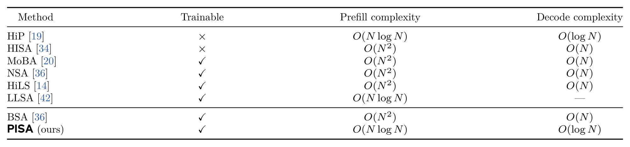
把这张表竖着看,结论很清楚:同时具备"可训练 + 预填充 $O(N\log N)$ + 解码 $O(\log N)$"的方法,表里只有 PISA 一行。$O(N\log N)$ 本身不是新东西(HiP 与 LLSA 都有),新的是把它做成一个可端到端训练的语言模型注意力层,并且给出解码路径的 $O(\log N)$ 保证。

一个容易被忽略的口径:PISA 的对照组 BSA 是作者用 NSA 的"selected-attention 分支 + 均值池化键摘要"重组的单层选择基线,并非某篇论文的原样复现;NSA 保留其学习式压缩分支与 selected-attention 分支;HiLS 保留其可学习 landmark 路由。训练时三种方法共享同一套数据、主干与注意力投影。(论文 §4.1 与 §C.1)

03 · Observation

观察:选择阶段为什么仍是二次的

把 $O(N^2/C)$ 拆开看很直观:每个 query 要看 $M=N/C$ 个块,共 $N$ 个 query,乘起来就是 $N^2/C$。分母上的 $C$ 只是把常数压小,不改变阶数。$N=256\text{K}$、$C=64$ 时 $\lceil N/C\rceil=4096$——每个 query 要做 4096 次块打分(推算),这正是长上下文里选块比注意力本身还贵的来源。

论文的出发点是:既然 $M$ 很大,那就别在叶块层平铺打分,而是先在一个"块数少得多"的粗粒度层上筛。粗层每个块覆盖的 token 多、块数少,筛完再只把幸存者的孩子展开——这正是 Figure 1 想表达的东西:

Figure 1 BSA 与 PISA 两种 Top-K 选择方式对比 — **Figure 1:** Comparison of two different Top-K selection methods for sparse attention. Top: BSA computes a score for each key block before performing Top-K selection. Bottom: PISA constructs a fine-to-coarse hierarchy of key blocks through mean pooling and expands only the selected candidates from coarse to fine during selection. Intermediate blocks are scored using LSE over their child summaries, while leaf blocks are scored using exact LSE over their original keys. **看图要点:**上图(BSA)里 $\ell=1$ 那一整条键带全部被标成"待打分候选"(蓝网纹),右侧写着"为所有块计算 Mean Score"——成本正比于块数。下图(PISA)同一个 $\ell=1$ 层里只有两个被橙色虚框圈出的块在打分,其余是"跳过计算"(白框);因为选择是从最上面的大块(橙虚线框,横跨整条键带)开始收窄的,越往上候选越少、越往下才展开。右侧两组说明对应两种打分:中间层用 **LSE over child-block**(对孩子摘要做 LSE),叶层用 **LSE over original keys**(对原始键做 LSE)。图例中"Selected by Top-K"是橙色虚框(被保留),"Selected KV"是橙色实心小格(最终真正参与注意力的键),两者一个是选择决策、一个是计算对象。报告 p.4

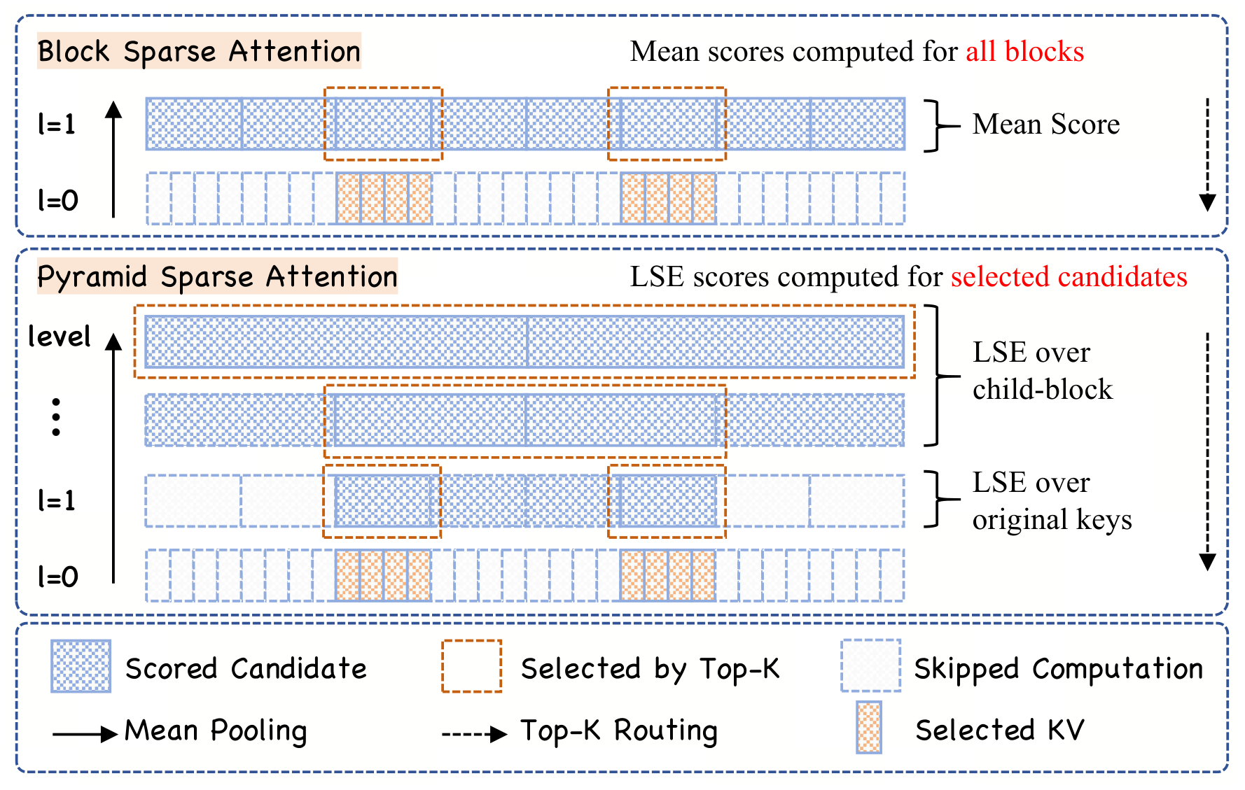
还有一处细节值得先记住:PISA 在每一层都问"这一层的候选数是不是已经不超过 $K$ 了?"如果是,直接全部保留、不打分。在粗层候选本来就少,$O(\log N)$ 层里最上面那几层几乎等于免费——这一点在后面的配置走查里会变成一个很漂亮的数字。

04 · Method

方法:金字塔键层级、由粗到细 Top-K 与 LSE 打分

4.1 由细到粗:建一座键的金字塔

层级是从精细往粗糙建的。第 0 层是原始键,$M_0=N$,每块就是一个 token;第 1 层是叶块,每 $C$ 个相邻 token 合成一块,于是 $M_1=\lceil N/C\rceil$;再往上每 $g=2$ 个相邻块合成一块:

$$M_{\ell+1}=\left\lceil\frac{M_\ell}{g_\ell}\right\rceil,\qquad g_0=C,\qquad g_\ell=g=2\;(\ell\ge 1) \tag{3}$$

每层的摘要由子块摘要均值池化得到,$\bar{k}_i^{(0)}=k_i$ 起步:

$$\bar{k}_i^{(\ell+1)}=\frac{1}{|\mathrm{Ch}_\ell(i)|}\sum_{r\in\mathrm{Ch}_\ell(i)}\bar{k}_r^{(\ell)},\qquad \ell\ge 0 \tag{4}$$

因为每一层的合并组大小相等,这个递推的结果就是"块内所有原始键的均值"。query 自始至终保持 token 粒度,不参与池化。

4.2 由粗到细:逐层收窄的 Top-K

选择方向与建塔方向相反。最粗层 $L$ 只有一个候选:

$$A_t^{(L)}=\{1\};\qquad s_t^{(\ell)}=\left[s_{t,i}^{(\ell)}\right]_{i\in A_t^{(\ell)}},\quad I_t^{(\ell)}=\mathrm{SelectK}\!\left(A_t^{(\ell)},s_t^{(\ell)}\right),\quad A_t^{(\ell-1)}=\bigcup_{i\in I_t^{(\ell)}}\mathrm{Ch}_{\ell-1}(i) \tag{5}$$

每层只处理上一层幸存块的孩子,候选规模被分支因子和预算双重卡住:

$$\left|I_t^{(\ell)}\right|\le K,\qquad \left|A_t^{(\ell-1)}\right|\le g\left|I_t^{(\ell)}\right|\le gK \tag{6}$$

一轮走完,$I_t^{(1)}$ 就是最终参与注意力的原始键值块。因为塔高是 $L=O(\log N)$,每层候选又是常数上界 $gK$,每个 query 的选路开销就是 $O(\log N)$,整段序列 $O(N\log N)$。这就是标题里"log-linear"的全部来源。

4.3 LSE 打分:为什么不用均值

剩下的问题是:中间层的块没有"原始键 LSE"可用,只有孩子摘要,该怎么打分?论文的答案是分数由孩子摘要上的 LogSumExp 给出:

$$s_{t,i}^{(\ell)}=\log\sum_{r\in\mathrm{Ch}_{\ell-1}(i)}\exp\!\left(\frac{q_t^{\top}\bar{k}_r^{(\ell-1)}}{\sqrt{d}}\right),\qquad \ell\ge 1 \tag{7}$$

叶层因为 $\bar{k}_r^{(0)}=k_r$,这个式子退化成对原始键的精确 LSE。每个候选最多摊开 $g$ 个中间孩子、或 $C$ 个原始键,所以打分成本也是有界的。

论文用泰勒展开说明这个选择不是随手取的。对进入打分的一批 logit $z_1,\dots,z_m$,设均值 $\bar z$、方差 $\mathrm{Var}(z)$:

$$s_{\mathrm{PISA}}=\log\sum_{j=1}^{m}e^{z_j}=\log m+\bar z+\tfrac{1}{2}\mathrm{Var}(z)+\text{higher-order terms} \tag{8}$$

丢掉 $\log m$,一阶截断就是"只取均值",二阶截断就是"均值 + 半个方差",这正好构成论文的两个消融变体:

$$s_{\mathrm{PISA-1}}=\bar z,\qquad s_{\mathrm{PISA-2}}=\bar z+\tfrac{1}{2}\mathrm{Var}(z) \tag{9}$$

再往深一步,附录 A 用 Jensen 不等式给出了一个"夹逼"关系。设块 $B$ 有 $g$ 个等大小的孩子 $C_1,\dots,C_g$,孩子摘要与 query 的点积记作 $m_j$,父块归一化后的真实 LSE 记作 $F_q(B)$:

$$\frac{1}{g}\sum_{j=1}^{g}m_j\;\le\;\hat F(B):=\log\!\left(\frac{1}{g}\sum_{j=1}^{g}e^{m_j}\right)\;\le\;F_q(B) \tag{10}$$

左边是 PISA-1 用的"均值平均",中间是 PISA 的分数(减去 $\log g$),右边是父块的真实 LSE。它说明:在孩子均值上做 LSE,比直接平均孩子均值更接近真实块质量,因为它保留并放大了孩子之间的差异;但它无法恢复每个孩子内部的方差,当孩子内部 logit 全相等时两端取等。

论文自己给这条论证加的边界:原文明确写道,式(10)比较的是"块分数的数值误差,并不保证获得更准确的块排序、也不保证能找回全局最高质量的叶块"(Appendix A.1)。所以这是"打分更贴近真值"的论证,不是"选择一定更正确"的定理。选择质量最终仍要靠实验证据——也就是后面 Table 7 的 Recall@8 诊断。

4.4 GQA 下的一次细微不一致

论文沿用 NSA 的做法:同一个 GQA 组内的 query head 共享同一组被选中的键块。PISA 把一个 KV head 下所有 query head 的 LSE 分数求和作为该块的分数:

$$u_{h,t,i}^{(\ell)}=\sum_{h'\in H(h)}s_{h',t,i}^{(\ell)} \tag{11}$$

但附录 A.3 指出,诊断实验里全注意力参考集是对块质量取平均,而 PISA 是对 query head 的 LSE 分数求和;即使 LSE 分数完全精确,这两种聚合规则也可能给出不同的块排序。这是一处论文主动披露的口径差异,不是错误,但读者看 Table 7 时应当知道。

05 · System

系统:Triton 内核、IO 账本与配置走查

算法本身是"每层打分-取 Top-K-展开"的循环,朴素实现会在层与层之间反复读写中间候选,把省下的 FLOPs 又还给显存带宽。论文的应对是把中间若干层融合进一个内核,候选索引全程留在寄存器/共享内存里,并且不物化任何密集的 query–key 分数矩阵。

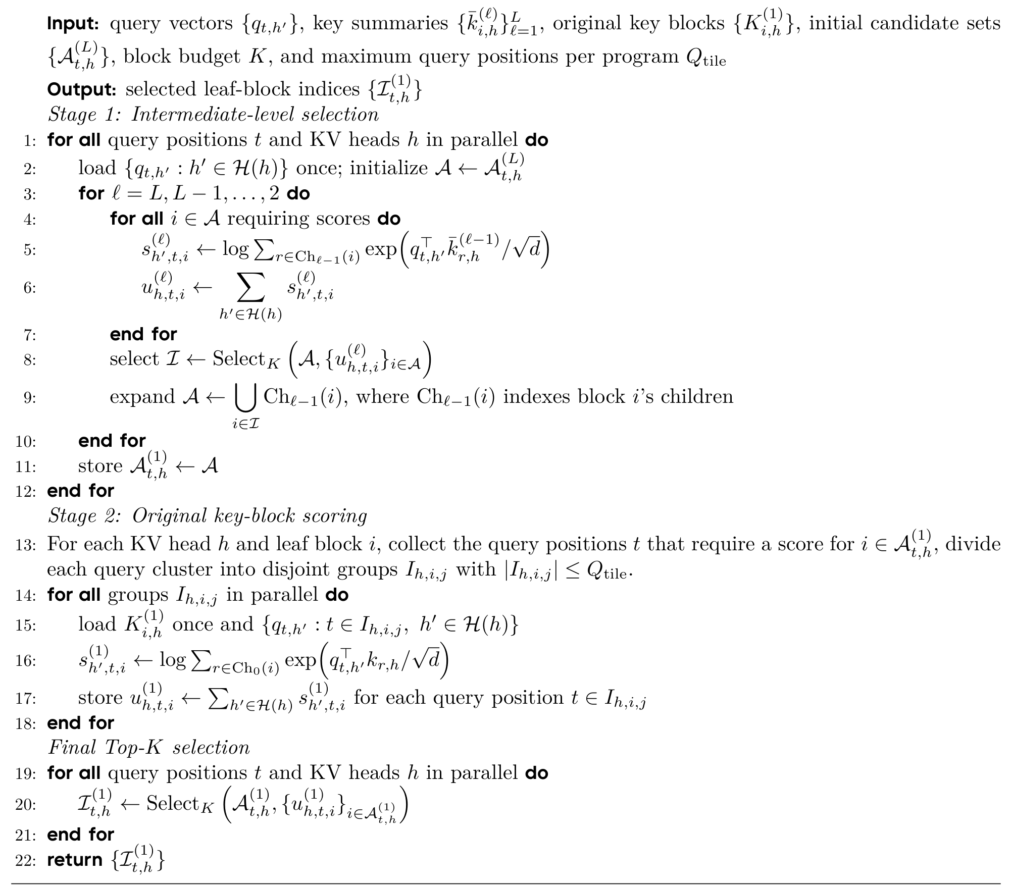
Algorithm 1 PISA 两阶段块选择算法 — **Algorithm 1:** Two-stage block selection for PISA. **逐步解读:**① **Stage 1(第 1–12 行)**按 (query 位置, KV head) 并行,query 向量只加载一次,然后从 $\ell=L$ 一路降到 $\ell=2$ 顺序处理中间层;第 5 行对每个候选算 LSE 分,第 6 行把一个 KV head 下所有 query head 的分数相加(即式 11),第 8 行取 Top-K,第 9 行把幸存块展开成孩子作为下一层候选。② **Stage 2(第 13–18 行)**换了并行维度:先按 (KV head, 叶块) 把需要该块分数的 query 聚成簇,每簇再切成至多 $Q_{\text{tile}}$ 个 query 的小组并行;第 15 行把键块 $K_{i,h}^{(1)}$ **只加载一次**,用它同时给一整组 query 打分——这就是"键块复用"。③ 最后(第 19–22 行)再起一个轻量内核,为每个 query 与 KV head 独立做最终 Top-K。④ 注意第 4 行与第 14 行的两个不同并行轴,这正是 Stage 1 与 Stage 2 的分工所在。报告 p.6

5.1 为什么训练用两阶段、解码用单阶段

论文没有停在"我们的内核很快",而是把两套设计的 IO 成本摆出来对账,这是全文最工程的一节。对单个 KV head,记一个 GQA 组里有 $G_Q$ 个 query head 共享同一个 KV head,键块大小 $C$,query 分块 $Q_{\text{tile}}$。

两阶段(训练/预填充):每个 query 关联至多 $gK$ 个候选键块,加载 query 的 IO 是 $O(NgKG_Qd)$;因为 query 分块并行,每个键块平均被加载

$$O\!\left(\frac{NgK}{(N/C)Q_{\text{tile}}}\right)=O\!\left(\frac{CgK}{Q_{\text{tile}}}\right)\ \text{次},\qquad\text{合计}\quad O\!\left(\frac{N\,CgKd}{Q_{\text{tile}}}\right) \tag{12}$$

于是两阶段的叶层 Q/K IO 总量是

$$O\!\left(NgKd\left(G_Q+\frac{C}{Q_{\text{tile}}}\right)\right) \tag{13}$$

单阶段要一次走到叶层,每个 query 直接加载至多 $gK$ 个原始键块,额外 IO 为 $O(NgKCd)$(式 14)。两者相比,只要

$$G_Q+\frac{C}{Q_{\text{tile}}}

两阶段就更省。论文的实现取 $G_Q=16$、$Q_{\text{tile}}=4$、$C=64$,代入得 $16+64/4=32<64$,条件成立,因此训练/预填充用两阶段。

解码时结论反过来。解码每步的簇里只有一个 query,没有跨 query 复用的空间:两阶段要加载 $gKC$ 个键、还要把 query 向量重复加载 $gK$ 次,IO 是 $O(gK(C+G_Q)d)$;单阶段可以直接复用中间层选择时已经加载过的 query,额外叶层 IO 只有 $O(gKCd)$。所以解码用单阶段融合内核,省掉重复加载 query 和额外的分组/终选内核启动。

这套账本的意义:它解释了一个容易被当成实现细节的设计选择——同一个算法在训练和解码下用了不同的内核结构,理由是可量化的 IO 而非直觉。判断条件是式(15)这一个不等式,换模型配置($G_Q$、$Q_{\text{tile}}$、$C$)时可以重新代入检验。

5.2 把配置落到具体层号上

抽象地讲"$O(\log N)$ 层、每层至多 $gK$ 个候选"容易滑过去。把它代进论文自己的两套训练配置(预训练 4K/$\;C=64$、$K=8$;继续预训练 16K/$\;C=64$、$K=32$,见 Table 5 与 §C.1),就能看见这座塔在真实长度上长什么样:

金字塔在论文两套配置下的逐层展开(依论文 §3.2、§4.1、§C.1 与 Table 5 的配置推算,非论文原表)
层级 $\ell$	每块覆盖 token	候选数 $\|A^{(\ell)}\|$	本层动作
$\ell=7$(最粗)	4096	1	候选数 ≤ $K$,直接全部保留,不打分
$\ell=6$	2048	2	不打分
$\ell=5$	1024	4	不打分
$\ell=4$	512	8	恰好等于 $K$,仍不打分
$\ell=3$	256	16	给 16 个候选打 LSE 分,留 8
$\ell=2$	128	16	给 16 个候选打 LSE 分,留 8
$\ell=1$(叶块)	64	16	对 16×64 = 1024 个原始键打分,留 8 块

左表为 4K 预训练配置($N=4096$,$C=64$,$K=8$,$g=2$):塔高 $L=\log_2(4096/64)+1=7$ 层。整条选路里真正需要打分的只有 2 个中间层(各 16 个候选),最后对 1024 个原始键打分,选出 8 个叶块 = 512 个键参与注意力。

同一座塔在 16K 继续预训练配置下的展开($N=16384$,$C=64$,$K=32$,$g=2$,推算)
层级 $\ell$	每块覆盖 token	候选数 $\|A^{(\ell)}\|$	本层动作
$\ell=9$(最粗)	16384	1	不打分
$\ell=8$	8192	2	不打分
$\ell=7$	4096	4	不打分
$\ell=6$	2048	8	不打分
$\ell=5$	1024	16	不打分
$\ell=4$	512	32	恰好等于 $K$,仍不打分
$\ell=3$	256	64	给 64 个候选打分,留 32
$\ell=2$	128	64	给 64 个候选打分,留 32
$\ell=1$(叶块)	64	64	对 64×64 = 4096 个原始键打分,留 32 块

塔高 $L=\log_2(16384/64)+1=9$ 层。最上面 6 层因为候选数不超过 $K=32$ 而完全免费;两个中间层各打分 64 个候选;叶层对 4096 个原始键打分后选出 32 个块 = 2048 个键。

这两张表还顺带解释了一件事:在 4K/8K 这种长度上,PISA 的免费层占了塔的大半,但叶层仍然固定要打分 $gK\cdot C$ 个原始键;而 BSA 此时只需要扫描 $M=N/C$ 个块摘要。当 $N/C$ 还小于 $gKC$ 时,BSA 的账更便宜——这就是下一节 Figure 3 里"4K–16K BSA 更快"的机制性原因。

「推算」的交换点:令"BSA 每 query 扫描的块摘要数 $N/C$"等于"PISA 每 query 在叶层打分的原始键数 $gKC$",得 $N=gKC^2$。代入 $g=2$、$K=8$、$C=64$ 得 $N\approx 65\text{K}$,即量级上交叉点应在 64K 附近;论文实测的交叉点落在 16K 与 32K 之间(Table 4)。两者同量级但不等,因为该式只比较了点积次数,没有计入 BSA 内核常数因子更低、PISA 中间层与融合内核的额外开销。这是本页的量级推算,不是论文结论。

5.3 其余工程约定

强制块与因果掩码:沿用 NSA 在 Flash Linear Attention(Yang & Zhang, 2024)中的默认策略,始终保留第一个、前一个、当前叶块及其祖先路径;预填充时当前块路径上的摘要可能含未来键,这些节点只保留、不用其分数参与排序;注意力内核另行屏蔽块内的未来 token。
反向传播:被选中的块索引在反向时固定,梯度只通过被选中的注意力条目流动,不穿过离散的选择决策。
解码缓存:金字塔缓存每 KV head 存 $O((N/C)d)$ 个元素,每层容量按固定比例扩容;即使每次扩容都整块拷贝,到长度 $N$ 的累计拷贝成本也只有 $O((N/C)d\log N)$,平均到每个生成 token 仍是 $O(\log N)$。

06 · Experiments

实验一:语言建模与下游任务

实验规模是 418M / 1.47B / 2.67B 三档,每档用同一套 decoder-only 主干与匹配的训练设置,100B token、序列长度 4096 从零预训练,再做 10B token 的 16K 继续预训练。稀疏方法统一 $C=64$,预训练 $K=8$、继续预训练 $K=32$。先把配置摊开看:

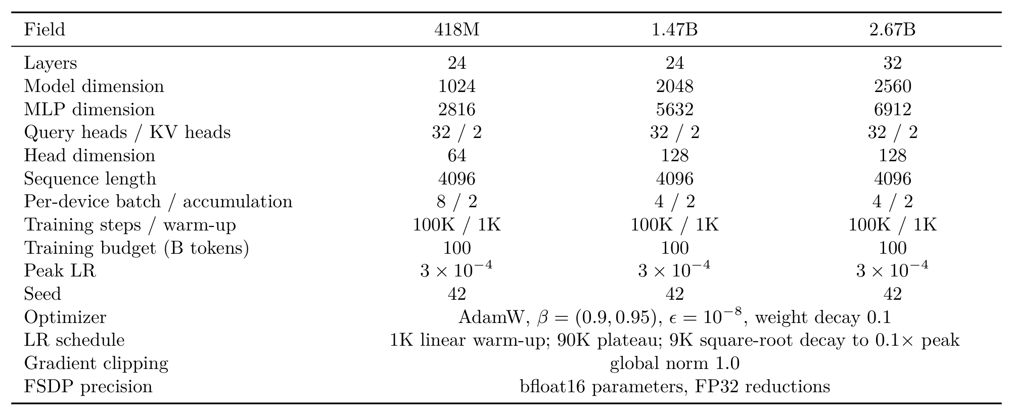
Table 5 从零预训练配置 — **Table 5:** From-scratch training configuration. **关键配置:**418M 是 24 层 / $d=1024$ / 头维 64;1.47B 是 24 层 / $d=2048$ / 头维 128;2.67B 是 32 层 / $d=2560$ / 头维 128。三档都是 **32 个 query head 对 2 个 KV head**,即 GQA 组大小 $G_Q=16$——这个数字直接决定了 §5.1 里 $G_Q+C/Q_{\text{tile}}=32$ 的 IO 不等式是否成立。预训练序列长度 4096、100K 步、100B token,峰值学习率 $3\times10^{-4}$,AdamW($\beta=(0.9,0.95)$、$\epsilon=10^{-8}$、weight decay 0.1),全局梯度裁剪 1.0,FSDP 用 bfloat16 参数 + FP32 归约,固定种子 42。三档共享同一套学习率日程:1K 线性预热、90K 平台、9K 平方根衰减到峰值的 0.1 倍。报告 p.19

其余未列在这张表里的设置:GPT-2 BPE 分词器(词表 50,257,补齐到 50,432 行)、pre-RMSNorm、SiLU 门控前馈、无 dropout;RoPE 只加在每个注意力头的高频一半维度上,基频 10,000(继续预训练时提到 80,000);继续预训练的 10B token 用 $3\times10^{-5}$ 预热 10% 再余弦衰减到 $3\times10^{-6}$,恢复模型参数与 Adam 优化器状态,packed 输入保留文档边界、不跨文档注意力。

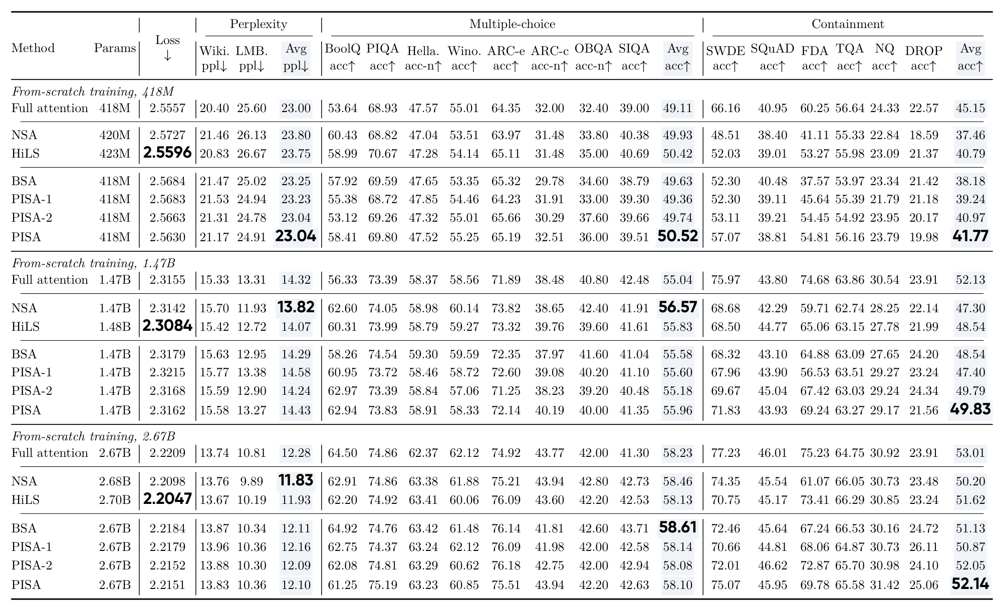
Table 2 语言建模与下游评测结果 — **Table 2:** Language modeling and downstream evaluation after 100B tokens of pretraining at 4K. Baselines include NSA [36] and HiLS [14]. Loss is the final training loss, and accuracies are reported as percentages. Gray columns show group averages; boldface marks the best sparse loss and group averages at each scale. **怎么读这张表:**横向分三块——困惑度(WikiText / LAMBADA 及其均值,越低越好)、八项多选题及其"Acc-8"均值、六项 containment 检索任务(SWDE / SQuAD / FDA / TQA / NQ / DROP)及其均值。"Containment"的判定标准是预测里包含任一标准答案(不区分大小写的字面子串)即可。三档规模各有一段:PISA 的 loss 在每一档都低于 BSA、PISA-1 与 PISA-2;containment 均值一栏,PISA 在 41.77 / 49.83 / 52.14 三个规模上**都是稀疏方法中的最高值**(加粗),但仍低于 Full Attention 的 45.15 / 52.13 / 53.01。报告 p.9

有一点必须照着原文的加粗位置说清楚,否则很容易读错:这张表里"最佳稀疏 loss"的加粗并不在 PISA 行,而在 HiLS 行(2.5596 / 2.3084 / 2.2047 三档都是)。论文正文的措辞也精确地避开了这一点——原话是 PISA "在三个规模上训练损失低于 PISA-1、PISA-2 和 BSA",而不是"低于所有稀疏方法"。事实核对如下(整理自 Table 2):

论文 Table 2 里"训练损失"这一列的逐档核对(数据取自论文 Table 2,整理)
规模	PISA	BSA	PISA-1	PISA-2	HiLS	NSA	论文加粗者
418M	2.5630	2.5684	2.5683	2.5663	2.5596	2.5727	HiLS
1.47B	2.3162	2.3179	2.3215	2.3168	2.3084	2.3142	HiLS
2.67B	2.2151	2.2184	2.2179	2.2152	2.2047	2.2098	HiLS

PISA 相对 BSA 的 loss 优势在三个规模上分别是 0.0054 / 0.0017 / 0.0033(本页相减,推算);相对 PISA-1/PISA-2 也一致更低,但幅度都在千分位。同一张表里 PISA 拿到加粗的是三个规模的 containment 均值,以及 418M 档的困惑度均值(23.04,与 PISA-2 并列)与 Acc-8 均值(50.52)。

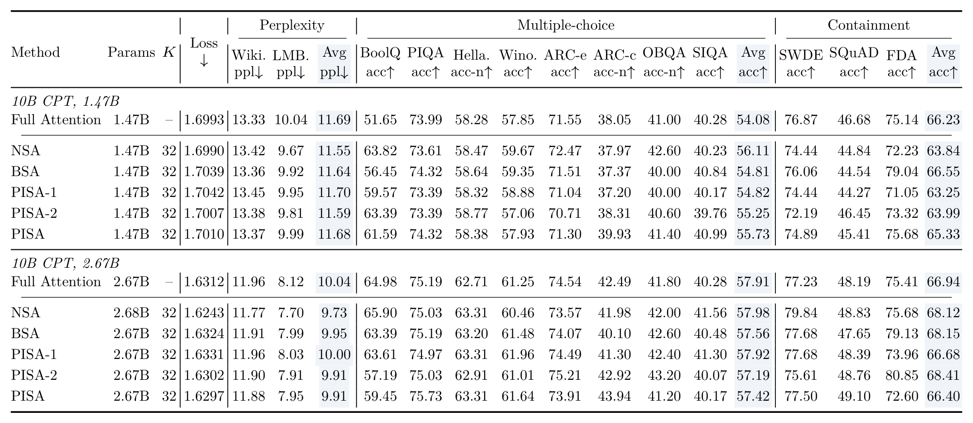
继续预训练(CPT)之后的口径变化值得单独提醒,因为这里有一个很容易踩的坑:

Table 6 16K 继续预训练后的下游结果 — **Table 6:** Training loss and downstream performance for the 1.47B and 2.67B models after 10B tokens of continued pretraining at 16K. Sparse methods, including NSA [36], use C = 64 and K = 32. Loss is the final training loss. Gray columns show group averages; the containment average covers SWDE, SQuAD Completion, and FDA. The block budget does not apply to Full Attention. **两个必须注意的口径差:**① **这张表的 containment 均值只覆盖 3 个任务**(SWDE / SQuAD / FDA),而 Table 2 是 6 个任务(多了 TQA / NQ / DROP),所以"Table 2 的 52.14"与"Table 6 的 66.40"**不能直接比大小**,它们不是同一个指标。② 继续预训练后 PISA 的 containment 均值(1.47B 为 65.33、2.67B 为 66.40)**低于 BSA**(66.55 / 68.15),论文正文也如实写了这一点。同时 PISA 的 loss 在 1.47B(1.7010)与 2.67B(1.6297)上都低于 BSA(1.7039 / 1.6324)与 PISA-1(1.7042 / 1.6331),论文的措辞即为此处。报告 p.20

建模质量部分的小结:PISA 在预训练阶段的检索类任务(containment)上稳定优于其他稀疏方法,损失与困惑度基本打平;但继续预训练之后 containment 反被 BSA 超过。论文摘要里"检索任务更好"的说法,主要依据是下一节的 RULER(Table 3),而不是 Table 6。

07 · Long-context & Efficiency

实验二:长上下文检索、选择质量与选择效率

7.1 RULER 大海捞针

长上下文用 RULER(Hsieh et al., 2024)的四个 needle-in-a-haystack 家族评测:单键、多键、多 query、多值,在 1K 到 16K 五个长度上贪心解码,用的是 16K 继续预训练后的 2.67B 模型。

Table 3 RULER 大海捞针结果 — **Table 3:** RULER needle-in-a-haystack results after 10B tokens of continued pretraining at 16K for the 2.67B models. Sparse methods use C = 64 and K = 32. Scores are accuracies in percent. The gray Avg column averages scores over the four task families at 1K, 2K, 4K, 8K, and 16K, before rounding. Boldface marks the best sparse result in each column. **读法与两个反直觉之处:**每个家族下有 1K/2K/4K/8K/16K 五列,最右的 Avg 是四个家族 × 五个长度的总平均。① 总平均一栏加粗的是 **PISA-2 的 62.92**,不是完整版 PISA 的 62.80——即在这个指标上"均值 + 半个方差"的二阶近似反而略高一点,差异很小但没有站在完整 LSE 一边。② 单键(niah_single)一栏的加粗几乎全被 **NSA** 拿走(16K 处 91.67,PISA 为 71.27),PISA 家族的优势集中在多键、多 query、多值这三个家族。③ 所有稀疏方法在 16K 的多键/多 query/多值上都出现明显衰减,最好的稀疏结果分别只有 15.20(多键,NSA)/ 25.20(多 query,PISA-2)/ 28.90(多值,NSA),与 Full Attention 的 23.13 / 34.85 / 57.20 相比,多 query 与多值两栏差距明显。报告 p.10

把 Table 3 里 16K 那一列单独摊平,能更清楚看到"谁在哪里更强"(对四个家族取算术平均,数据取自 Table 3,推算):PISA 30.86、PISA-2 32.56、PISA-1 28.09 均高于 BSA 的 25.90,但都低于 NSA 的 39.99 与 Full Attention 的 53.50。也就是说,PISA 相对 BSA 的检索优势在 16K 处仍然成立,但它并不是这一列的最强者。

7.2 选择质量诊断

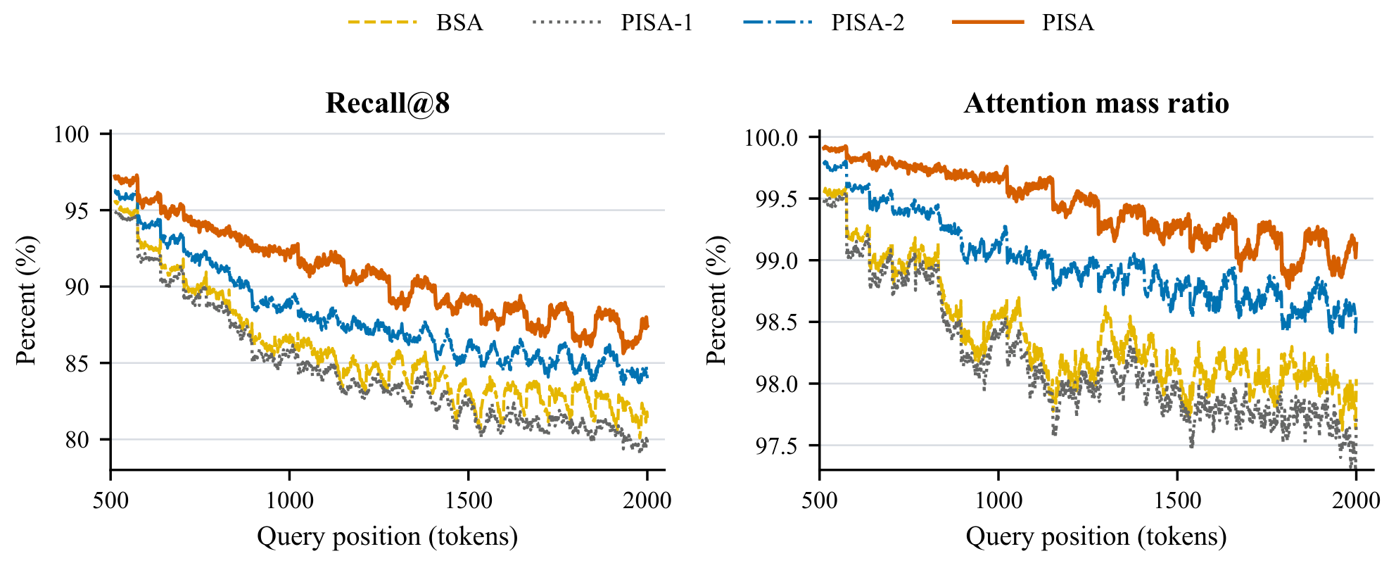
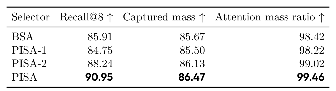
这一节回答的是"金字塔 + LSE 到底选得准不准"。实验设计很干净:拿一个 418M 的全注意力模型(100B token 预训练),用同一份 query/key 张量,让各选择器各自选 $K=8$ 个块,然后和全注意力权重导出的参考集对比;24 层全用,$C=64$,100 条 FDA prompt,只看 query 位置 $\ge 512$(此时可选的块超过 8 个)。两个指标分别是集合重合度 Recall@K 和保留注意力质量占比 MassRatio。

Figure 2 选择质量随 query 位置的变化 — **Figure 2:** Block-selection quality on 100 FDA prompts using identical Full-Attention queries and keys. Curves show mean Recall@8 and attention mass ratio by query position. All selectors and the reference share K = 8 and the forced-block policy; Recall@8 includes forced blocks. **曲线解读:**左图 Recall@8,右图注意力质量比,横轴是 query 位置(500–2000 token)。橙色实线(完整 PISA)在两张图里都**全程位于最上方**;蓝点划线是 PISA-2、灰色点线是 PISA-1、黄色虚线是 BSA。三条 LSE/均值线的排序在两张图里一致:PISA > PISA-2 > PISA-1 ≈ BSA(右图里 PISA-1 与 BSA 几乎重合,BSA 甚至略高)。两条曲线都随 query 位置**单调下降**:序列越长、可选的块越多,任何单层或层次选择器都更难命中全注意力最看重的块。注意 Recall@8 里含三个强制块(首块/前块/当前块),所以曲线起点很高(近 95%),下降部分才反映选择能力。报告 p.10

Table 7 选择质量聚合结果 — **Table 7:** Block-selection quality on 100 FDA prompts using shared Full-Attention queries and keys, with C = 64 and K = 8. Scores are percentages, averaged over query rows with more than eight eligible blocks. Recall@8 includes the three forced blocks. Boldface marks the best result in each column. **四个选择器在三个指标上的聚合结果:**PISA 拿到全部三项加粗——Recall@8 90.95%(对比 BSA 85.91%、PISA-1 84.75%、PISA-2 88.24%)、保留注意力质量 86.47%(BSA 85.67%)、注意力质量比 99.46%(BSA 98.42%)。这里可以读出两层信息:其一,完整 LSE 明显优于一阶近似 PISA-1(90.95 vs 84.75),说明"保留孩子之间的方差"这个二阶信息确实是选择质量的主要来源;其二,注意力质量比一栏所有方法都在 98% 以上,说明被选中的块几乎能覆盖参考集所覆盖的注意力质量,各选择器在这一指标上的差距被压缩了。报告 p.21

7.3 选择延迟

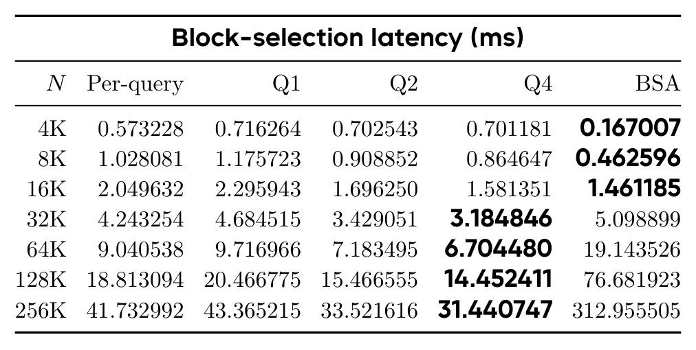
最后是效率。评测对象是选块这一个阶段的延迟:随机 BF16 的 query/key、batch 1、32 个 query head、2 个 KV head、$d=64$、$C=64$、$K=8$、$g=2$,点积在 FP32 累加,计时包含均值摘要构建与全部选择阶段,不含被选中块上的稀疏注意力计算。

Figure 3 预填充选块延迟对比 — **Figure 3:** Prefill block-selection latency from 4K to 256K with C = 64 and K = 8. Timings include mean-summary construction and all selection stages, but exclude attention over the selected blocks. The key-block reuse implementation of PISA uses Q_tile = 4; annotations show speedups over BSA. Complete settings are provided in Appendix B. **三条曲线与交叉点:**黄色虚线是 BSA,灰色点线是 PISA 的 per-query 融合实现,橙色实线是键块复用实现($Q_{\text{tile}}=4$,即论文的 Q4)。① **交叉点是这张图最重要的信息**:4K–16K 区间 BSA 反而更快(16K 处 BSA 1.461 ms vs Q4 1.581 ms),从 32K 起 Q4 反超并一路拉开,64K/128K/256K 分别快 2.86×/5.31×/9.95×。② BSA 在长序列上的曲线呈明显上翘(256K 达 312.96 ms),正是 $O(N^2/C)$ 项在起作用。③ 键块复用相对 per-query 实现的增益在 64K–256K 稳定在 1.30×–1.35×,幅度不大但方向一致——这正是 §5.1 里 $G_Q+C/Q_{\text{tile}}=32<64$ 那个不等式带来的收益。报告 p.11

Table 4 定长选块延迟明细 — **Table 4:** Fixed-length block-selection latency from 4K to 256K. Q1, Q2, and Q4 reuse one leaf-key tile across up to one, two, and four query references, respectively. Boldface marks the lowest latency at each sequence length. **逐列对照:**Q1/Q2/Q4 是键块复用程度不同的三个实现(每个叶键块分别服务 1/2/4 个 query)。加粗位置标出了每行的最优:4K、8K、16K 三行是 **BSA** 最快(0.167007 / 0.462596 / 1.461185 ms);32K 到 256K 四行是 Q4 最快(3.184846 / 6.704480 / 14.452411 / 31.440747 ms)。另外注意 4K 处 Q4(0.701181 ms)比 per-query(0.573228 ms)慢——论文正文明确解释了原因:序列短时候选块少,"把 query 分组以复用键块"的组织开销超过了复用带来的收益,从 8K 起才转为正收益。报告 p.18

效率部分的小结:这是一张"赢在长序列"的成绩单。选择阶段的复杂度从 $O(N^2/C)$ 变成 $O(N\log N)$ 之后,收益要等到 $N$ 足够大才盖过 PISA 固定多出来的那部分开销;论文实测的交叉点在 16K–32K 之间,而 256K 时是近 10 倍的差距。对于本页读者最关心的两个问题——"它比 BSA 快吗"(长序列上快很多,短序列上慢)和"快多少"(选块阶段 9.95×;端到端倍数论文未测量,见 §8.3)——答案都在这一节。

08 · Commentary

补充与点评:技术来源、边界与未披露项

8.1 局限(论文自述)

论文的 Limitations 只有一段,内容非常克制:计算资源限制了所探索的模型规模与预训练数据预算,而这两者都会显著影响性能以及相对基线的增益;在已评测的配置内,核心结论——金字塔块选择在保持竞争力的同时降低了选择复杂度——成立。除此之外论文没有自述其他局限。

8.2 技术来源一览

把论文里每个组件对应的上游标注单独整理出来,能更清楚看出哪些是继承、哪些是本代改造:

技术来源一览(据论文行内引用整理,非论文原表;引用为论文自己的标注口径,本页未逐条核对参考文献条目)
组件	论文标注的上游	本代的改造 / 集成
两阶段块稀疏框架(选块 + 选中块上算注意力)	BSA 通用范式,论文归到 MoBA(Lu et al., 2025)与 NSA(Yuan et al., 2025)	沿用两阶段划分;第一阶段由"平铺扫全部块"改为"金字塔逐层收窄"
池化块摘要用于选择	MoBA(Lu et al., 2025)、InfLLM-V2(Zhao et al., 2025)的 query-dependent 摘要	不只用叶块摘要,而是把它扩展成 $O(\log N)$ 层的摘要金字塔
多级 / 由粗到细选择	HiP(Lee et al., ICLR 2025,免训练)在多级上重复选择;LLSA(Zhou et al., CVPR 2026)为扩散 Transformer 做层次 Top-K	首次把它做成可训练的语言模型注意力层,并补上解码路径的 $O(\log N)$ 论证
块打分函数	无直接上游(BSA/NSA 类方法用摘要点积或均值)	改为子块摘要上的 LogSumExp;附录 A 用 Jensen 不等式给出"均值平均 ≤ 摘要 LSE ≤ 父块真实 LSE"的夹逼论证,并派生出 PISA-1/PISA-2 两个泰勒截断变体
GQA 组内共享选择	NSA(Yuan et al., 2025)	沿用;把组内各 query head 的 LSE 分求和(附录 A.3 指出这与诊断中参考集的"取平均"口径不一致,可能产生不同排序)
强制块策略(首块 / 前一块 / 当前块)与解码单阶段结构	沿用 NSA 在 Flash Linear Attention(Yang & Zhang, 2024)中的默认实现	沿用掩码与强制块语义;解码把中间层与叶层融合进单个内核
训练 / 预填充的两阶段 Triton 内核与键块复用	本文工作	Stage 1 融合全部中间层、候选索引不出内核;Stage 2 按 (KV head, 叶块) 聚簇、每个键块只加载一次服务至多 4 个 query
评测协议	lm-evaluation-harness(Biderman et al., 2023)、BASED / JRT(Arora et al., 2024)的 containment 实现、RULER(Hsieh et al., 2024)	全套沿用;containment 用前三个任务(或六个,见 Table 2 与 Table 6 的口径差)

8.3 未披露、值得补测的点

端到端速度与吞吐。Figure 3 与 Table 4 测的都是选块阶段的延迟,并明确排除被选中块上的稀疏注意力计算;全文未给出训练/推理的步时、tokens/s 或端到端加速比,也未给出显存占用实测。因此"9.95× 更快"是选择阶段的口径,不能直接当作端到端收益。评测硬件型号也未披露(全文未提 GPU 型号)。
64K 以上的建模质量。256K 长度只出现在选块延迟微基准里,用的是随机 query/key,没有真实模型在 64K–256K 上的困惑度或检索评测。而 PISA 的复杂度优势恰恰要到这些长度才显现,所以"长序列更快"有实测支撑,"长序列仍然好用"目前只有 16K 以内的证据。
金字塔的维护开销未单独计量。计时已包含摘要构建,但除 Figure 3 这一项外,论文没有报告金字塔缓存在训练与解码中的额外显存、也没有与 BSA 做显存对比。摘要金字塔每 KV head 是 $O((N/C)d)$ 元素,量级不大,但缺实测。
单种子,无误差棒。三个规模的训练与评测都固定 seed 42,Table 2/3/6 的差异多在千分位到个位数百分点之间(例如 RULER 总平均 PISA 62.80 vs PISA-2 62.92 vs NSA 61.07),未做重复实验或显著性检验,小差距的稳定性待观察。
基线覆盖范围。可训练对照组只有 BSA、NSA、HiLS 三家。Table 1 中列入的 MoBA(Lu et al., 2025)与参考文献里的 SeerAttention、IndexCache、LongCat、InfLLM-V2 等均未参与实测;免训练方法是否能在同长度上给出更低延迟也未对照。
LSE 与截断近似的胜负并不一致。完整 PISA 在 Table 7 诊断(PISA 90.95 vs PISA-2 88.24)与 Table 2 损失上都胜出,但在 Table 3 的 RULER 总平均上是 PISA-2(62.92)略高于 PISA(62.80)。论文未讨论这一反转;若要主张"精确 LSE 更好",RULER 这一项需要补充说明或重复验证。
强制块对诊断指标的贡献。Recall@8 里含三个必然命中的强制块,论文在 Figure 2 图注中如实标注了这一点,但未给出剔除强制块后的净 Recall,读者难以直接判断"8 个槽位里有 3 个是送的"之后选择器自身的命中率。

8.4 总体评价

贡献的实质。块稀疏注意力的选择阶段是二次的这个瓶颈,在长上下文系统里是真实存在的工程问题,而这篇论文给出的是一个结构清晰、代价可分析的解法:用池化建塔把"扫全部块"换成"逐层收窄"。$O(N\log N)$ 这个复杂度本身在此之前已经有免训练方法(HiP)和扩散模型方法(LLSA)触及,所以本文的核心增量在于三处:把层次化选择做进可训练的语言模型注意力层、把块打分从均值换成 LSE 并给出夹逼论证、以及把训练/预填充与解码的 IO 账本算清楚并落成两套 Triton 内核。第三点尤其扎实——式(13)(15)那种"代入 $G_Q=16$、$Q_{\text{tile}}=4$、$C=64$ 看不等式成不成立"的写法,比常见的"我们的内核经过充分优化"要有信息量得多。

证据的强度。实验的分工是清楚的:建模质量用三个规模和 100B+10B token 的训练来支撑,选择质量用同一份张量上的对照诊断来支撑,选择效率用 4K–256K 的微基准来支撑。三块证据各自都能自圆其说,但拼起来并不构成"PISA 全面更优"的结论:损失被 HiLS 压着,单键检索被 NSA 压着,RULER 总平均被自家的 PISA-2 压着,继续预训练后的 containment 被 BSA 压着,16K 以内选块延迟被 BSA 压着。PISA 真正的、在所有实验里都成立的强项只有两项:六个 containment 任务的均值(预训练阶段,三个规模全部最高),以及 32K 以上的选块延迟(64K 起 2.86×,256K 到 9.95×)。论文摘要的措辞("常识推理相当、检索更好")基本对应这两项,没有过度外推,这一点是诚实的。

适用边界。这套机制的价值随序列长度增长,在 16K 以内它甚至更慢;它的设计目标场景是长上下文预填充与长序列解码。如果读者的部署长度在 4K–16K,这篇论文给不出采用理由;如果落在 64K 以上,那么"选择阶段随长度二次增长"这件事确实会被这张方法解决掉,而它的质量代价在 16K 的实验里看起来是可以接受的。

还没有回答的问题。最关键的一个是:选块阶段快 10 倍,端到端快多少?这取决于被选中块上的稀疏注意力计算占比。论文没有测,因此这项收益能兑现多少仍是开放问题。次关键的是:金字塔维护的显存与拷贝开销在真实训练循环里是否真的可以被 $O(\log N)$ 平摊吸收,以及 64K 以上质量是否守得住——这两点都需要超出本文配置的实测。

Glossary

术语速查

阅读中遇到缩写,可随时回到这里;正文里的缩写也可悬停查看释义。

阅读术语表(正文中带虚线下划线的缩写悬停可见)
缩写	全称	一句话解释
PISA	Pyramid Sparse Attention	本文提出的块稀疏注意力:金字塔键层级 + 由粗到细的逐层 Top-K 选择。
BSA	Block Sparse Attention	块稀疏注意力的通称;本页中特指论文的对照组——用均值池化摘要做单层 Top-K 选择的基线。
Top-K 选择	Top-K Selection	从候选块里保留分数最高的 $K$ 个。$K$ 是块预算,论文预训练取 8、继续预训练取 32。
LSE	LogSumExp	$\log\sum_j e^{z_j}$。注意力权重归一化里的分母,也是"一个块对 query 有多重要"的连续度量。
叶块	Leaf Block	金字塔第 1 层,$C$ 个相邻原始键合成一块,是真正参与注意力计算的单位。
分支因子 $g$	Branching Factor	上一层多少个块合成上一层的一个块。论文中 $g_0=C$、$g_\ell=2$($\ell\ge1$)。
GQA	Grouped-Query Attention	多个 query head 共享一个 KV head(Ainslie et al., 2023)。本文中同组 query head 共享同一组被选中的块。
$G_Q$	Query heads per KV head	一个 KV head 对应的 query head 数。论文配置为 32/2,故 $G_Q=16$。
$Q_{\text{tile}}$	Query tile size	Stage 2 里每个键块一次复用服务的 query 数上限,论文取 4。
PISA-1 / PISA-2	First- / Second-order variants	把 LSE 泰勒展开分别截断到一阶(仅均值)和二阶(均值 + 半个方差)的消融变体。
CPT	Continued Pre-Training	继续预训练。本文在 4K 预训练之后用 10B token 把序列长度扩到 16K、$K$ 扩到 32。
RoPE	Rotary Position Embedding	旋转位置编码。本文只加在每个头的高频一半维度上,继续预训练时基频从 10,000 提到 80,000。
FSDP	Fully Sharded Data Parallel	全分片数据并行。本文用 bfloat16 参数 + FP32 归约。
RULER	—	长上下文评测套件(Hsieh et al., 2024)。本文用其中四个大海捞针家族,1K–16K 五个长度。
Containment	Containment Accuracy	生成结果只要包含任一标准答案(不分大小写的字面子串)即判对,用于检索类任务。
Recall@K	—	选出块与全注意力参考块的重合比例,含三个强制块。Table 7 中 PISA 为 90.95%。
Attention mass ratio	注意力质量比	选出块覆盖的注意力质量 ÷ 参考集覆盖的质量。Table 7 中 PISA 为 99.46%。
Triton	—	面向 GPU 的类 Python 内核编程语言,本文的训练/预填充与解码内核均用它实现。