Overview: the claim and the key numbers
The paper attacks a narrow, load-bearing problem: block-sparse attention saves the attention computation but not the cost of deciding which blocks to keep. The conventional recipe scores every query against all $N/C$ key blocks, so the selection stage costs $O(N^2/C)$ in total — attention itself has become linear while block selection stays quadratic, and at long sequence lengths selection becomes the new bottleneck. PISA replaces the full scan with a pyramid: keys are mean-pooled into $O(\log N)$ levels, and selection walks from the coarsest level down, expanding only the survivors. Routing drops to $O(\log N)$ per query and $O(N\log N)$ over the sequence.
The argument in three steps
Problem. Block-sparse attention runs in two stages: pick $K$ key blocks per query, then attend only inside them. Stage two is linear, but stage one must score all $N/C$ block summaries per query, so it stays $O(N^2/C)$ overall. The longer the sequence, the more block selection looks like full attention again.
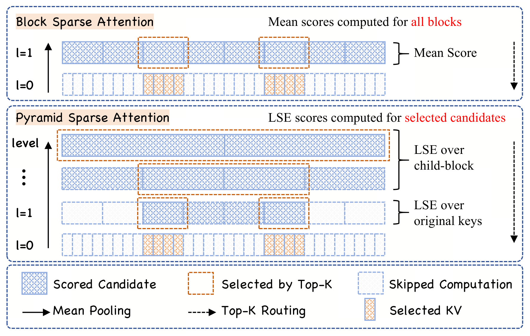
Method. Pool keys into a fine-to-coarse pyramid ($C$ per group, then 2 per group), then select in the opposite direction: at each level score only the children of blocks kept at the previous level, keep the top $K$, and expand. Candidates per level are bounded by $gK$ and there are $O(\log N)$ levels, giving $O(\log N)$ routing per query. The block score is a LogSumExp over child summaries rather than an average of child means; Appendix A sandwiches it between the mean score and the parent's true raw-key LSE.
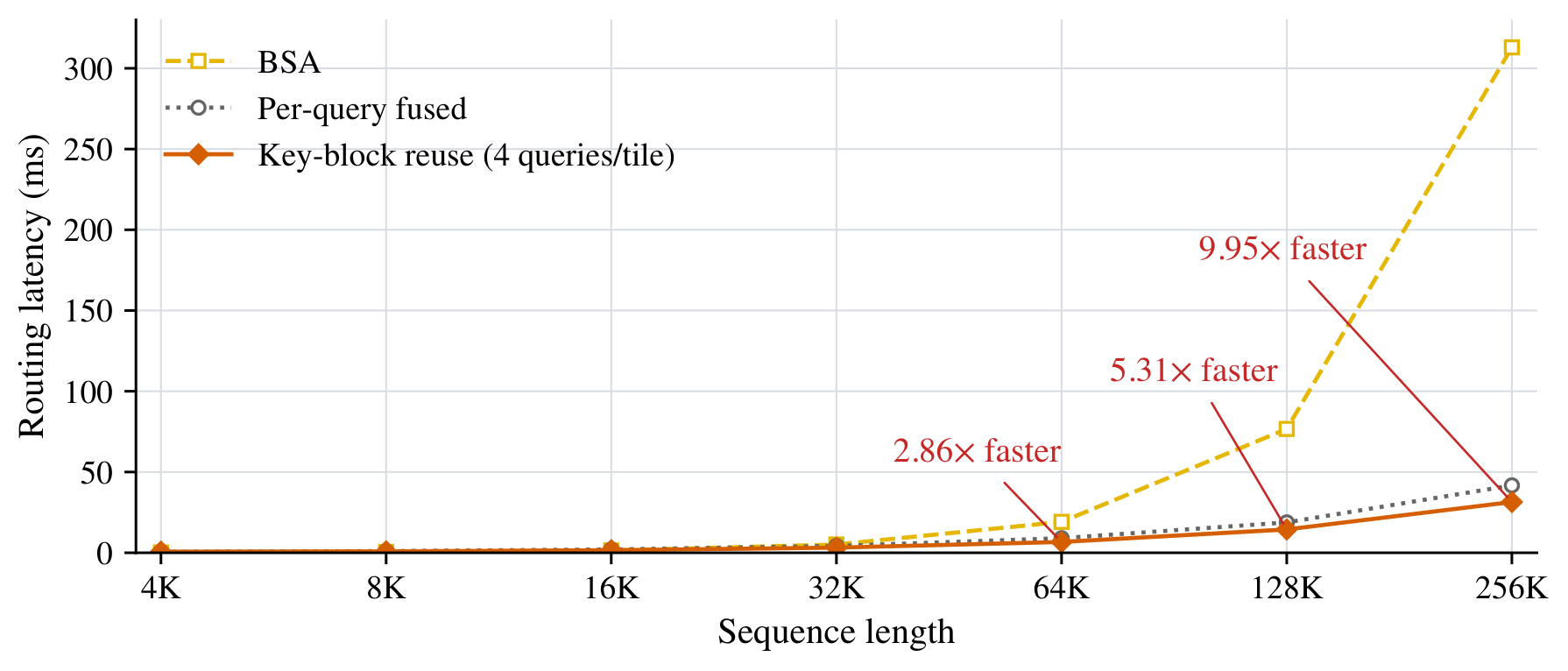
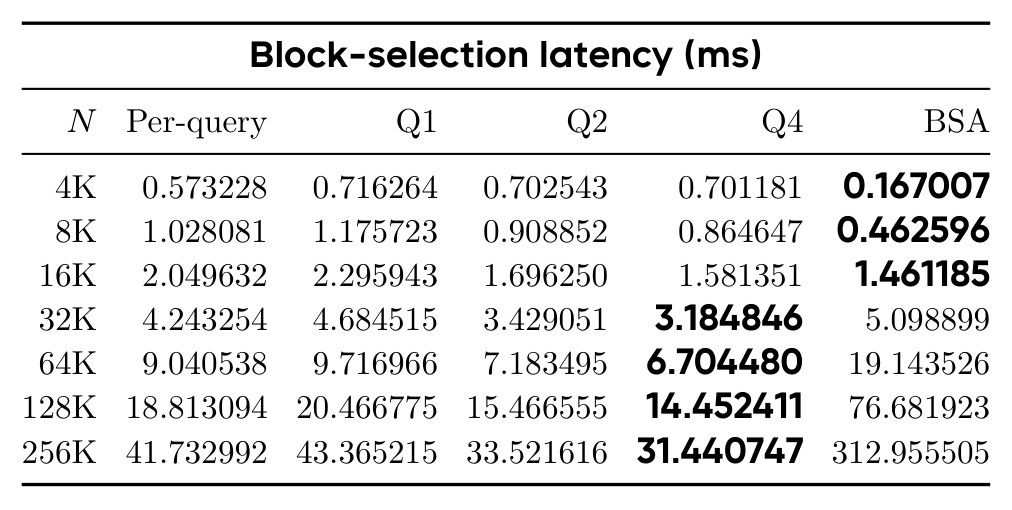
Evidence. At 418M / 1.47B / 2.67B, pretrained on 100B tokens at 4K and continued-pretrained on 10B tokens at 16K, language-modelling loss and commonsense reasoning are comparable to BSA, NSA and HiLS; the six-task containment average is the best among sparse methods at all three scales; the RULER average is clearly above BSA. Selection latency overtakes BSA after 32K and is 9.95× faster at 256K.
Background: two stages, and the bottleneck in the first
Self-attention grows quadratically with sequence length, which is the hard wall in long-context modelling. Sparse attention lets each query see only part of the keys; the block-sparse variant groups keys and values into contiguous blocks of $C$ tokens, which keeps the sparse computation inside regular tiled kernels instead of turning it into scattered gathers.
The paper formalises block-sparse attention as two stages. Stage one gives each key block a summary vector $\bar{k}_i=f(K_i)$ — mean pooling or a learned projection — and scores it against the query:
Stage two attends over the original keys and values inside the selected blocks:
Each query reads at most $KC$ keys, so stage two is $O(N)$. Stage one, however, scores $M=N/C$ blocks per query, accumulating $O(N^2/C)$: the attention cost was cut, the selection cost was not.
Where this sits relative to prior work
The paper positions the literature on two axes — trainable or not, and prefill/decode complexity. The table is worth reading line by line, because it names both PISA's niche and its competitors:
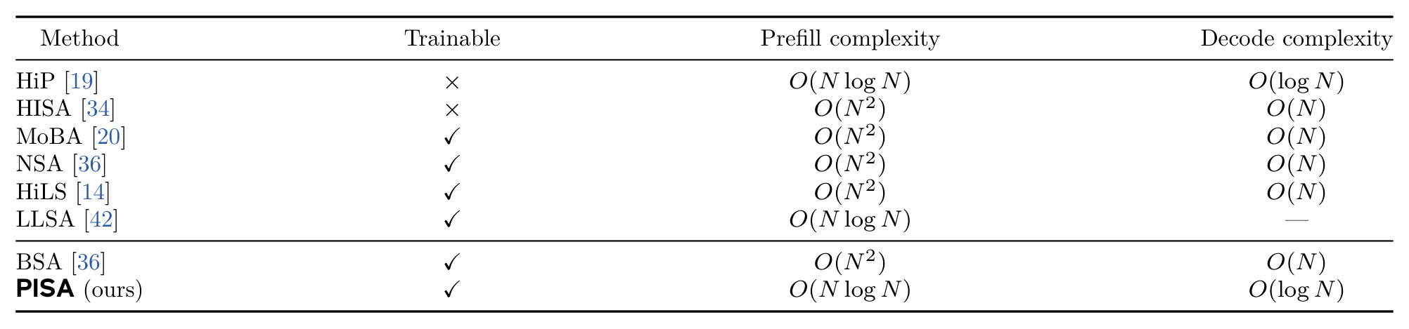
Read down the columns and the claim is sharp: the only row that is simultaneously trainable, $O(N\log N)$ at prefill and $O(\log N)$ at decode is PISA. Log-linear complexity itself is not new — HiP and LLSA both have it — the contribution is making it an end-to-end trainable language-model attention layer with a decode path that keeps the $\log N$ guarantee.
Method: a pyramid of keys, selected coarse-to-fine
3.1 Fine to coarse: building the pyramid
Level 0 is the raw keys ($M_0=N$, one token per block); level 1 is the leaf blocks ($M_1=\lceil N/C\rceil$); above that every $g=2$ adjacent blocks merge:
Summaries are mean-pooled from their children, starting from $\bar{k}_i^{(0)}=k_i$:
Because the merge groups are equally sized at every step, the recursion yields the mean of all original keys in the block. Queries stay token-level throughout; they are never pooled.
3.2 Coarse to fine: narrowing the Top-K
Selection runs in the opposite direction. The coarsest level has a single candidate, and each level only processes the children of the previous level's survivors:
After the walk, $I_t^{(1)}$ is the set of original key/value blocks used for attention. The pyramid is $L=O(\log N)$ levels tall and each level is capped at $gK$ candidates, so routing costs $O(\log N)$ per query and $O(N\log N)$ over the sequence — the "log-linear" in the title.
One detail carries a lot of weight: if a level has at most $K$ candidates, they are all retained without scoring. The top levels of the pyramid are therefore nearly free, which is what makes the mechanism cheap in practice and not just asymptotically.
💡 Click any image to open the original 300 DPI version; click again or press Esc to close.
Scoring: LogSumExp, and why not the mean
Intermediate blocks have no raw keys available, only child summaries. The paper scores them with a LogSumExp over those summaries:
At the leaf level $\bar{k}_r^{(0)}=k_r$, so this degenerates into the exact LSE over original keys. Each candidate expands at most $g$ intermediate children or $C$ raw keys, so scoring stays bounded.
A Taylor expansion explains the choice. For logits $z_1,\dots,z_m$ with mean $\bar z$ and variance $\mathrm{Var}(z)$:
Dropping $\log m$, truncating at first order gives "mean only" and at second order "mean plus half the variance" — exactly the two ablation variants:
Appendix A then gives a Jensen sandwich. Let block $B$ have $g$ equally sized children $C_1,\dots,C_g$, let $m_j$ be the dot product of the query with child $j$'s summary, and let $F_q(B)$ be the parent's normalised raw-key LSE:
The left term is the mean-of-means used by PISA-1, the middle term is PISA's score minus $\log g$, and the right term is the parent's true LSE. In words: taking a LogSumExp over child means sits closer to the true block score than averaging the child means does, because it preserves and amplifies differences between children. It cannot recover variation inside a child; when all logits within a child are equal the bounds meet.
4.1 An inconsistency the paper discloses
Following NSA, query heads inside one GQA group share the selected blocks. PISA sums their LSE scores into a single block score:
Appendix A.3 points out that the full-attention reference in the diagnostic instead averages block masses across those heads. Even with exact LSE scores, summing and averaging can rank blocks differently. The paper flags this itself; it is a convention mismatch to keep in mind when reading Table 7, not an error.
Systems: Triton kernels and the IO ledger
Naively, the level-by-level loop would write and re-read intermediate candidates and give back in memory bandwidth what it saved in FLOPs. The paper's answer is to fuse the intermediate levels into a single kernel, keep candidate indices local to the program, and never materialise a dense query–key score matrix.
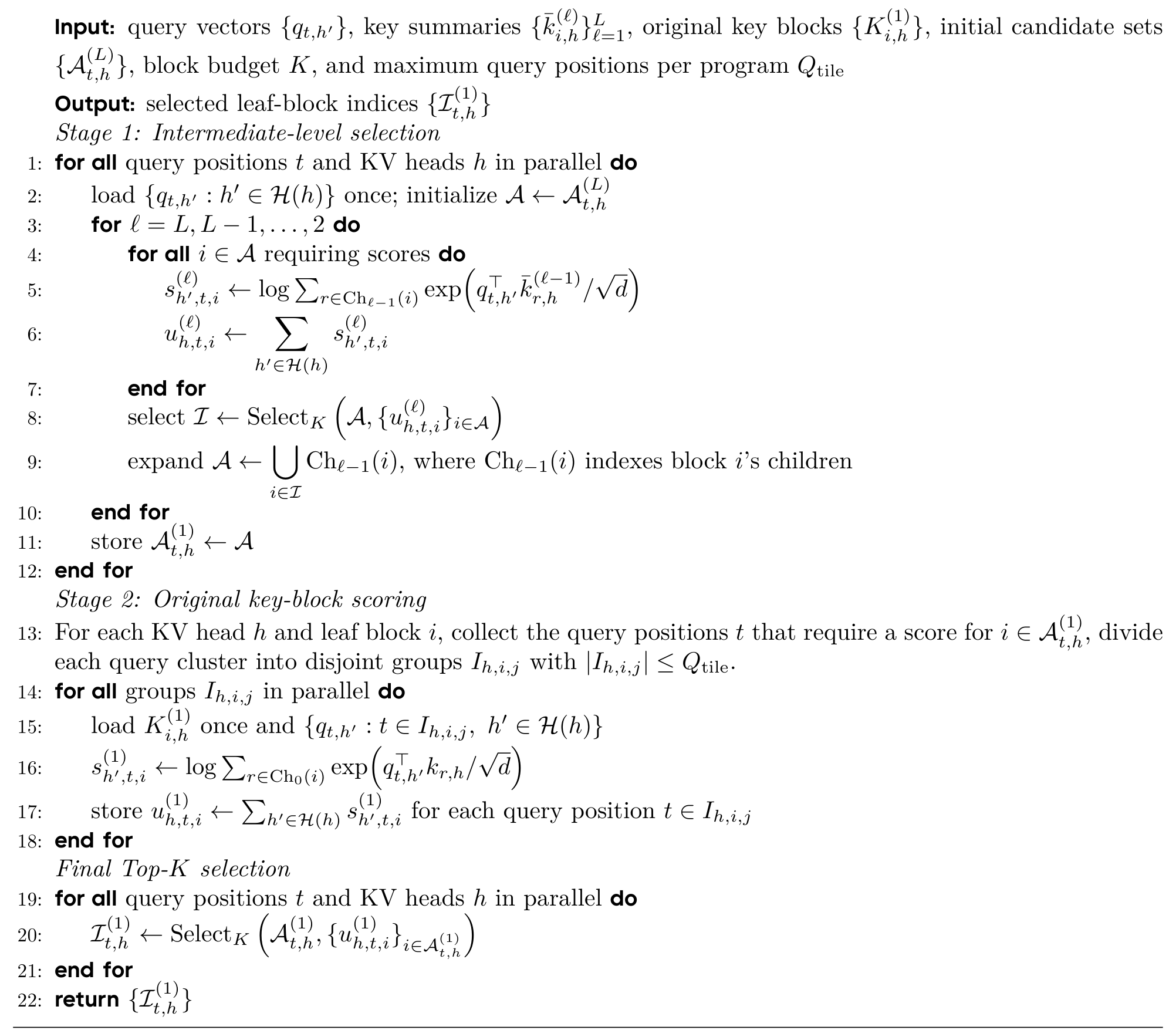
5.1 Why training uses two stages and decoding one
Rather than asserting that the kernels are fast, the paper puts the two designs' IO costs side by side. Per KV head, let $G_Q$ query heads share it, $C$ be the block size and $Q_{\text{tile}}$ the query tile.
Two-stage (training/prefill). Each query is tied to at most $gK$ candidate key blocks, so loading its queries costs $O(NgKG_Qd)$; because query tiles run in parallel, each key block is loaded on average $O(CgK/Q_{\text{tile}})$ times, giving a total key IO of $O(NCgKd/Q_{\text{tile}})$. The two-stage leaf-level Q/K IO is therefore
Single-stage walks straight to the leaf level, loading up to $gK$ original key blocks per query, for an extra $O(NgKCd)$ (Eq. 13). The two-stage design wins whenever
With the implementation's $G_Q=16$, $Q_{\text{tile}}=4$ and $C=64$, this is $16+64/4=32<64$ — the condition holds, so training and prefill use the two-stage kernel.
Decoding flips the conclusion. A decoding cluster contains a single query, so there is no cross-query reuse: the two-stage kernel would load $gKC$ keys and reload the query vectors $gK$ times, costing $O(gK(C+G_Q)d)$, while a single-stage kernel reuses the queries already loaded during intermediate selection and needs only $O(gKCd)$. Hence the fused single-stage selector for decoding, which also avoids separate grouping and final-selection launches.
5.2 Following the configuration down to actual levels
"$O(\log N)$ levels, at most $gK$ candidates each" is easy to skim past. Substituting the paper's own two training configurations (pretraining at 4K with $C=64$, $K=8$; continued pretraining at 16K with $C=64$, $K=32$) shows what the pyramid actually looks like at realistic lengths:
| Level $\ell$ | Tokens per block | Candidates $|A^{(\ell)}|$ | What happens |
|---|---|---|---|
| $\ell=7$ (coarsest) | 4096 | 1 | at most $K$, retained without scoring |
| $\ell=6$ | 2048 | 2 | no scoring |
| $\ell=5$ | 1024 | 4 | no scoring |
| $\ell=4$ | 512 | 8 | exactly $K$ — still no scoring |
| $\ell=3$ | 256 | 16 | 16 LSE scores, keep 8 |
| $\ell=2$ | 128 | 16 | 16 LSE scores, keep 8 |
| $\ell=1$ (leaf) | 64 | 16 | $16\times64$ = 1024 raw keys scored, keep 8 blocks |
The pyramid is $L=\log_2(4096/64)+1=7$ levels tall. Only two intermediate levels require scoring (16 candidates each), and the leaf level scores 1024 raw keys to pick 8 blocks — 512 keys attended.
| Level $\ell$ | Tokens per block | Candidates $|A^{(\ell)}|$ | What happens |
|---|---|---|---|
| $\ell=9$ (coarsest) | 16384 | 1 | no scoring |
| $\ell=8$ | 8192 | 2 | no scoring |
| $\ell=7$ | 4096 | 4 | no scoring |
| $\ell=6$ | 2048 | 8 | no scoring |
| $\ell=5$ | 1024 | 16 | no scoring |
| $\ell=4$ | 512 | 32 | exactly $K$ — still no scoring |
| $\ell=3$ | 256 | 64 | 64 candidates scored, keep 32 |
| $\ell=2$ | 128 | 64 | 64 candidates scored, keep 32 |
| $\ell=1$ (leaf) | 64 | 64 | $64\times64$ = 4096 raw keys scored, keep 32 blocks |
Here $L=9$. The top six levels are entirely free because candidates never exceed $K=32$; two intermediate levels score 64 candidates each; the leaf level scores 4096 raw keys and keeps 32 blocks — 2048 keys attended.
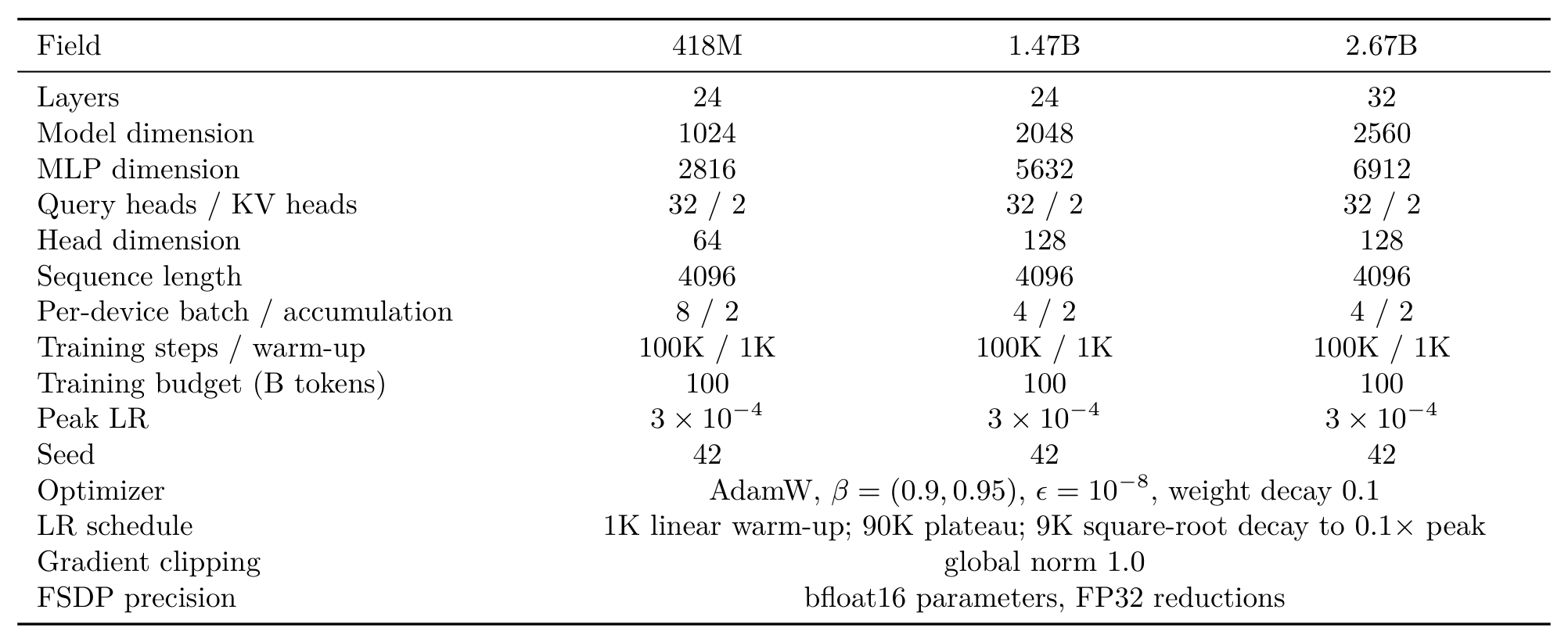
These two tables also explain why BSA wins at short lengths: at 4K the leaf level still scores a fixed $gK\cdot C$ raw keys, while BSA only has to scan $M=N/C$ block summaries. While $N/C Three scales — 418M / 1.47B / 2.67B — share one decoder-only backbone per scale and matched training settings: 100B tokens at sequence length 4096 from scratch, then 10B tokens of 16K continued pretraining. Sparse methods use $C=64$ throughout, with $K=8$ for pretraining and $K=32$ for continued pretraining (CPT). The configuration first: Settings not in that table: GPT-2 BPE tokenizer (vocabulary 50,257 padded to 50,432), pre-RMSNorm, SiLU-gated feed-forward, no dropout; RoPE applied only to the high-frequency half of each attention head with base 10,000 (raised to 80,000 for continued pretraining); the 10B-token continued-pretraining run warms up to $3\times10^{-5}$ over the first 10% of steps and cosine-decays to $3\times10^{-6}$, restoring model parameters and Adam state, with packed inputs preserving document boundaries and no cross-document attention. One point has to be stated according to where the paper's own boldface actually sits, or the table is easy to misread: the bold "best sparse loss" is not in the PISA row — it is in the HiLS row (2.5596 / 2.3084 / 2.2047 at the three scales). The paper's prose is careful to match: it claims PISA has lower loss than PISA-1, PISA-2 and BSA, not lower than every sparse baseline. [organized] from Table 2: PISA's loss advantage over BSA is 0.0054 / 0.0017 / 0.0033 across the three scales (subtracted on this page, [estimated]); it is also consistently below PISA-1 and PISA-2, but every gap is in the third decimal. What PISA does take in bold on this table is the containment average at all three scales, plus the perplexity average (23.04, tied with PISA-2) and the Acc-8 average (50.52) at 418M. The change of convention after continued pretraining deserves its own warning, because it is an easy trap: Long-context retrieval uses four RULER needle-in-a-haystack families (Hsieh et al., 2024) — single-key, multi-key, multi-query and multi-value — greedily decoded at five lengths from 1K to 16K, on the 2.67B models after 16K continued pretraining. Flattening the 16K column of Table 3 makes the picture clearer (arithmetic mean over the four families, values from that table, [estimated]): PISA 30.86, PISA-2 32.56 and PISA-1 28.09 all beat BSA's 25.90, but all sit below NSA's 39.99 and Full Attention's 53.50. PISA's retrieval edge over BSA holds at 16K; it is not the strongest method in that column. This section answers whether the pyramid plus LSE actually selects the right blocks. The design is clean: take a 418M full-attention model (100B tokens pretrained), feed every selector the same query and key tensors, let each pick $K=8$ blocks, and compare against a reference set derived from the full-attention weights. All 24 layers, $C=64$, 100 FDA prompts, query positions $\ge512$ only (where more than eight blocks are eligible). The two metrics are the overlap Recall@K and the retained attention mass ratio. Finally, efficiency. What is measured is the latency of the selection stage alone: random BF16 queries and keys, batch 1, 32 query heads, 2 KV heads, $d=64$, $C=64$, $K=8$, $g=2$, dot products accumulated in FP32. Timings include mean-summary construction and all selection stages and exclude attention over the selected blocks. The Limitations section is one short paragraph: computational constraints limited the model sizes and pretraining budgets explored, and both factors can substantially affect performance and the relative gains over baselines; within the settings evaluated, the central finding — pyramid block selection reduces selection complexity while keeping performance competitive — holds. No other limitation is self-reported. Separating each component's upstream attribution makes it clear what is inherited and what is this paper's own change: What the contribution really is. Quadratic block selection is a real engineering bottleneck in long-context systems, and the paper answers it with a structure that is both simple and analysable: build a pooling pyramid and replace "scan every block" with "narrow level by level". The $O(N\log N)$ complexity itself had already been reached by a training-free method (HiP) and by a diffusion-model method (LLSA), so the incremental contribution is threefold: putting hierarchical selection inside a trainable language-model attention layer, replacing the block score with an LSE backed by a sandwich argument, and working out the IO ledger for training/prefill versus decoding and turning it into two Triton kernels. That third point is the most solid — writing out "substitute $G_Q=16$, $Q_{\text{tile}}=4$, $C=64$ and check whether the inequality holds" is far more informative than the customary claim that a kernel is well optimised. How strong the evidence is. The division of labour is clear: modelling quality rests on three scales and 100B+10B tokens of training, selection quality on a controlled diagnostic over identical tensors, and selection efficiency on a 4K–256K microbenchmark. Each strand stands on its own, but together they do not add up to "PISA is better across the board." Loss is beaten by HiLS; single-key retrieval is beaten by NSA; the RULER average is beaten by PISA's own PISA-2 variant; containment after continued pretraining is beaten by BSA; selection latency below 16K is beaten by BSA. What holds in every experiment is narrower: the six-task containment average during pretraining (best at all three scales) and selection latency above 32K (2.86× from 64K, 9.95× at 256K). The abstract's phrasing — comparable commonsense reasoning, better retrieval — maps onto exactly those two, and does not overreach. That is an honest abstract. Where it applies. The value of the mechanism grows with sequence length; below 16K it is outright slower. Its target is long-context prefill and long-sequence decoding. A reader deploying at 4K–16K gets no reason to adopt it from this paper; at 64K and beyond, the fact that selection grows quadratically with length is genuinely removed, and the quality cost at 16K looks acceptable in these experiments. What is still open. The most important question is: if selection is 10× faster, how much faster is the end-to-end forward pass? That depends on the share of time taken by attention over the selected blocks, and the paper does not measure it, so how much of the benefit is realised remains open. Next is whether the pyramid's memory and copying overhead is really amortised as $O(\log N)$ inside a real training loop, and whether quality holds beyond 64K — both need measurements outside this paper's configuration. Abbreviations are also hoverable in the prose via dotted underlines.5.3 Remaining conventions
Experiments: language modelling and downstream
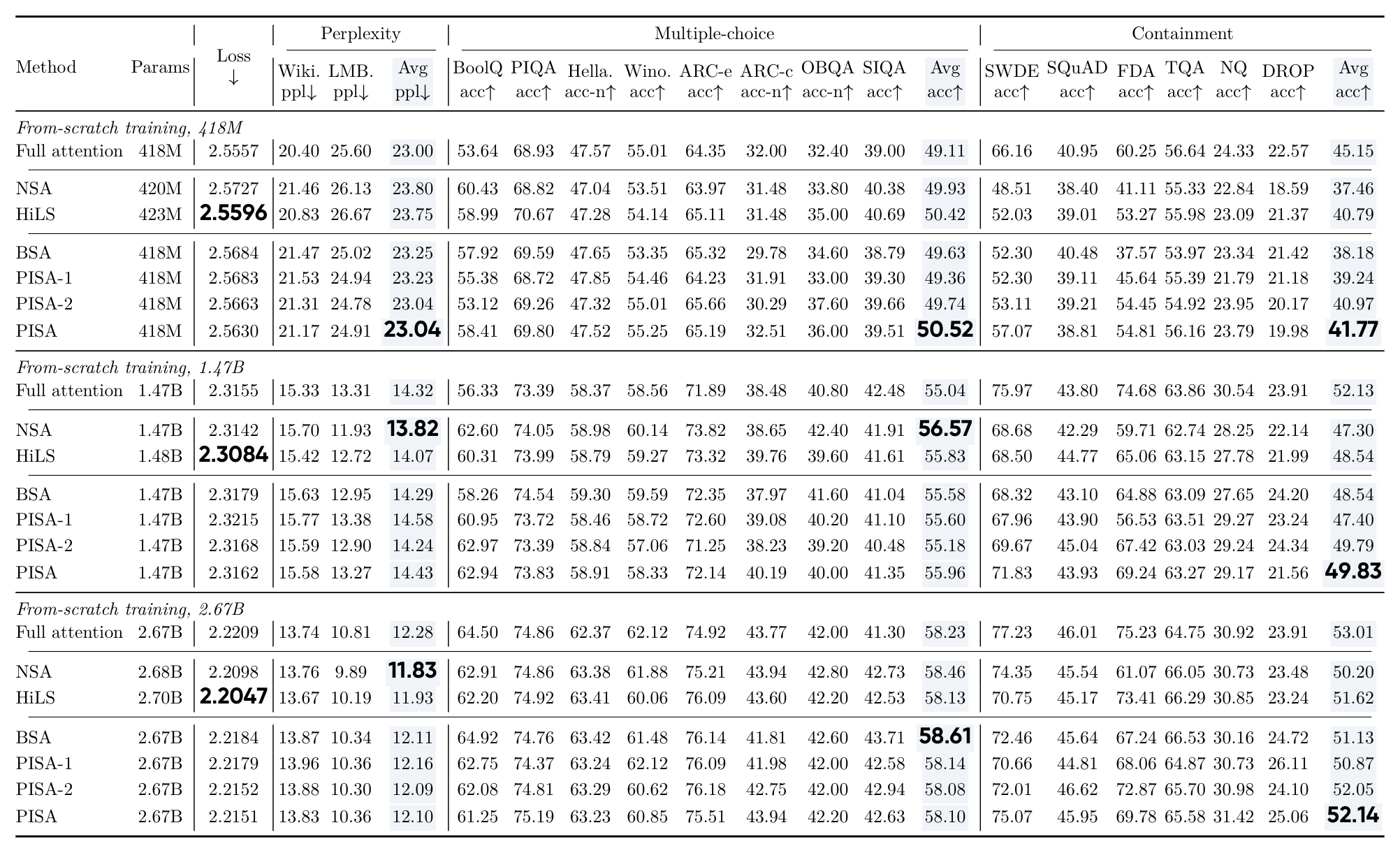
Scale PISA BSA PISA-1 PISA-2 HiLS NSA Bold in the paper 418M 2.5630 2.5684 2.5683 2.5663 2.5596 2.5727 HiLS 1.47B 2.3162 2.3179 2.3215 2.3168 2.3084 2.3142 HiLS 2.67B 2.2151 2.2184 2.2179 2.2152 2.2047 2.2098 HiLS 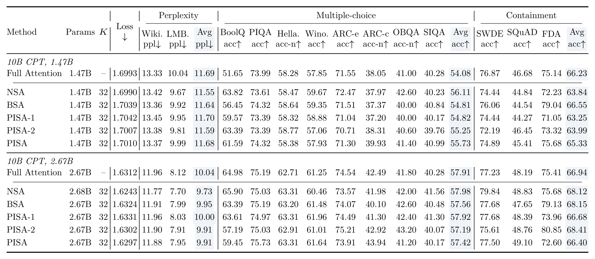
Long context, selection quality, selection efficiency
7.1 RULER needle-in-a-haystack

7.2 Block-selection diagnostic
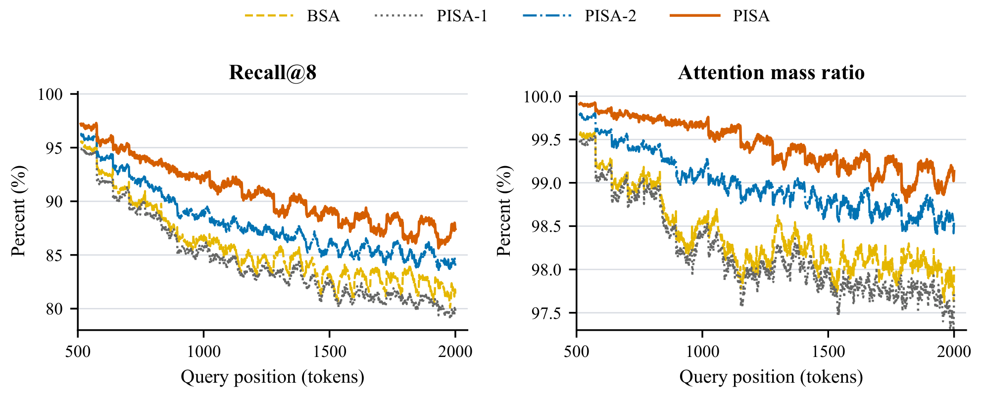
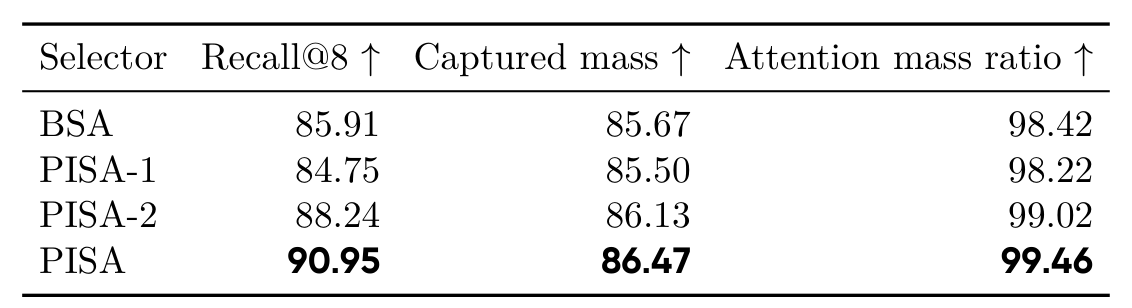
7.3 Selection latency
Commentary: lineage, limits, and what is not disclosed
8.1 Limitations (the paper's own)
8.2 Where the components come from
Component Upstream as attributed by the paper Change / integration in this work Two-stage block-sparse framework (select, then attend inside) General BSA paradigm, attributed to MoBA (Lu et al., 2025) and NSA (Yuan et al., 2025) Keeps the two stages; stage one changes from a flat scan over all blocks to a level-by-level narrowing Pooled block summaries for selection Query-dependent summaries in MoBA (Lu et al., 2025) and InfLLM-V2 (Zhao et al., 2025) Extends a single leaf-level summary into a pyramid of $O(\log N)$ summary levels Multi-level / coarse-to-fine selection HiP (Lee et al., ICLR 2025, training-free) repeats selection across levels; LLSA (Zhou et al., CVPR 2026) does hierarchical Top-K for diffusion transformers First to make it a trainable language-model attention layer, with an $O(\log N)$ argument for the decode path Block scoring function No direct upstream (BSA/NSA-family methods use summary dot products or means) LogSumExp over child summaries; Appendix A proves the sandwich "mean of means ≤ summary LSE ≤ parent raw-key LSE" and derives the PISA-1 / PISA-2 Taylor variants from it Shared selection within a GQA group NSA (Yuan et al., 2025) Kept; the per-head LSE scores are summed (Appendix A.3 notes the diagnostic reference instead averages, so the two can rank blocks differently) Forced-block policy (first / previous / current) and the decode-stage structure NSA's default implementation in Flash Linear Attention (Yang & Zhang, 2024) Masking and forced-block semantics kept; decoding fuses intermediate and leaf levels into one kernel Two-stage Triton kernels and key-block reuse for training/prefill This work Stage 1 fuses all intermediate levels with candidate indices staying on-chip; Stage 2 clusters by (KV head, leaf block) and loads each key block once to serve up to 4 queries Evaluation protocol lm-evaluation-harness (Biderman et al., 2023), the BASED / JRT containment implementations (Arora et al., 2024), RULER (Hsieh et al., 2024) Adopted as-is; containment uses three tasks or six depending on the table (see the Table 2 / Table 6 convention gap) 8.3 Not disclosed, worth testing next
8.4 Assessment
Glossary
Term Full name One-line explanation PISA Pyramid Sparse Attention This paper's method: a pyramid of key levels plus coarse-to-fine level-by-level Top-K selection. BSA Block Sparse Attention The general family; on this page it means the paper's baseline — single-level Top-K over mean-pooled summaries. Top-K selection — Keep the $K$ highest-scoring candidate blocks. $K$ is the block budget: 8 for pretraining, 32 for continued pretraining. LSE LogSumExp $\log\sum_j e^{z_j}$ — the denominator of the softmax, and a continuous measure of how much a block matters to a query. Leaf block — Level 1 of the pyramid: $C$ adjacent raw keys, the unit that actually takes part in attention. Branching factor $g$ — How many blocks of a level merge into one block of the next. Here $g_0=C$ and $g_\ell=2$ for $\ell\ge1$. GQA Grouped-Query Attention Query heads share KV heads (Ainslie et al., 2023). Here, heads in a group share one selected block set. $G_Q$ Query heads per KV head 32 query heads over 2 KV heads in this paper, so $G_Q=16$. $Q_{\text{tile}}$ Query tile size How many queries one loaded leaf key block serves in Stage 2; the implementation uses 4. PISA-1 / PISA-2 First- / second-order variants Taylor truncations of the LSE score: mean only, and mean plus half the variance. CPT Continued Pre-Training After 4K pretraining, 10B more tokens extend the length to 16K and the budget to $K=32$. RoPE Rotary Position Embedding Applied to the high-frequency half of each head only; base raised from 10,000 to 80,000 for continued pretraining. FSDP Fully Sharded Data Parallel Used with bfloat16 parameters and FP32 reductions. RULER — Long-context evaluation suite (Hsieh et al., 2024); four needle-in-a-haystack families at 1K–16K here. Containment Containment accuracy Correct if the generation contains any gold answer as a case-insensitive literal substring; used for retrieval tasks. Recall@K — Overlap between selected and full-attention reference blocks, forced blocks included. PISA scores 90.95%. Attention mass ratio — Mass covered by the selected blocks divided by the reference set's mass. PISA scores 99.46%. Triton — Python-like kernel language for GPUs; both the training/prefill and decoding kernels are written in it.