Paper Reading · Elastic Attention: Test-time Adaptive Sparsity Ratios

01 · Overview

Overview: Elastic Attention in One Page

Long-context inference is dominated by attention cost. The standard remedy is hybrid attention: some heads keep full attention (FA) for accuracy, the rest run sparse attention (SA) for speed. But the FA/SA ratio is usually a fixed, pre-deployment constant — while the paper's preliminary study (§2) shows that tasks differ by an order of magnitude in how much sparsity they tolerate. So why not let the model decide, per input, how sparse to be? Elastic Attention adds a lightweight Attention Router (0.27M params/layer) that assigns every KV head to FA or SA at inference time. Trained for 12 hours on 8×A800 with a fully frozen backbone, it lets 4B/8B models match or beat full-attention baselines on long-context benchmarks.

Reading conventions: every number on this page follows the paper; anything this page organizes or converts from the paper's configuration is flagged as [organized] or [estimated]. Notation follows the paper: FA=full attention, SA=sparse attention, $\Omega_{\text{MSR}}$=model sparsity ratio (share of sparse heads), $\Omega_{\text{ESR}}$=effective sparsity ratio (accounts for each head's pruning rate), $t$=target sparsity during training.

Training budget

12 hours · 8×A800backbone frozen; only the router trains

Router overhead

+0.27M params/layerhead dim 128; avg. latency 0.196 ms

Training data

0.74B tokens8K–64K sequences, 5 sources

Test-time sparsity

$\Omega_{\text{MSR}}$ 0.63–0.85input-adaptive: code ~0.82, QA ~0.63–0.68

Inference speedup

1.51× – 3.28×FA-XA / XA-SSA, RULER 256K

Evaluation

3 backbones × 3 long-context suitesQwen3-4B/8B, Llama-3.1-8B-Instruct

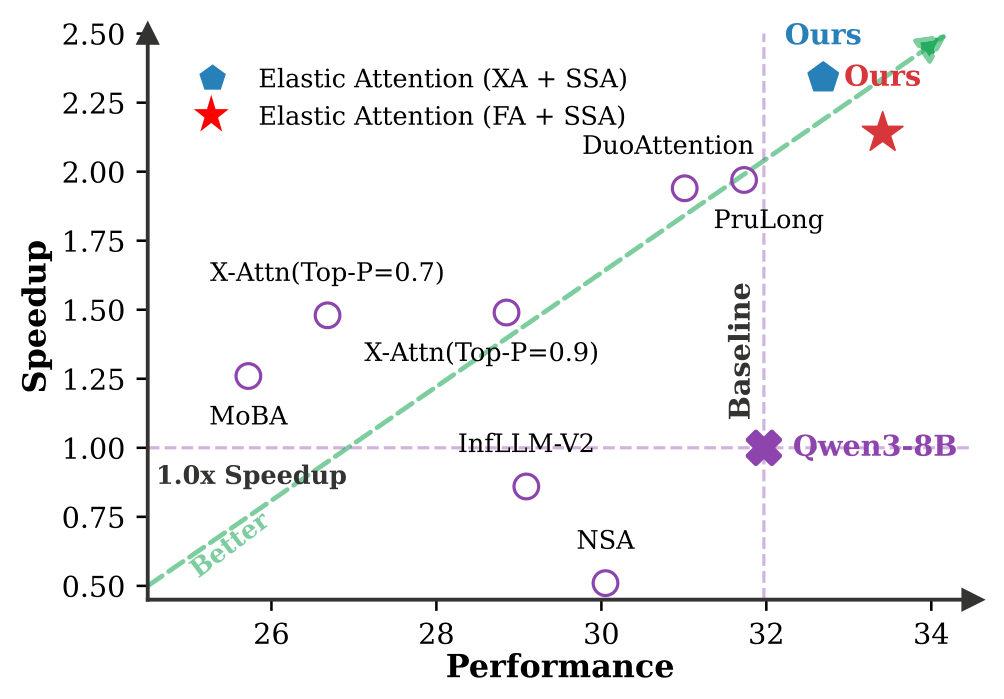
The opening figure puts adaptive sparsity on the table — same model, two settings, compared with existing sparse-attention methods:

Figure 1: Elastic Attention vs existing approaches on LongBench-V2 — **Figure 1:**Comparison between Elastic Attention (ours) and existing approaches on LongBench-V2 (Bai et al., 2025). “(XA+SSA)” and “(FA+SSA)” denote our different settings. The two settings: FA-SSA keeps retrieval heads on full attention while the rest stream sparsely; XA-SSA implements even the retrieval heads with XAttention's training-free block sparsity, pushing the whole model into the fully sparse regime — one guards accuracy, the other chases throughput. Exact axis definitions are in the paper; per-length readings appear in Figure 8 and Table 2. The paper also notes that methods such as NSA and InfLLM-V2 impose architectural constraints on KV head counts (e.g., multiples of 16) that do not align with Llama-3.1-8B, whereas Elastic Attention leaves the backbone untouched. Report p.1

💡 Click any image to open the full-resolution version; click again or press Esc to close.

Takeaway: three moves — ①observe: downstream tasks split into sparsity-robust and sparsity-sensitive regimes; ②route: a tiny Attention Router assigns each KV head to FA/SA per input, trained with Gumbel-Softmax + straight-through estimation; ③deploy: one fused kernel executes both head types in a single pass. Together they replace a static ratio with a per-request one.

02 · Background & Observation

Background: FA, SA, and the hybrid-head bound

Full attention enjoys quadratic cost; sparse attention cuts it by keeping only a fraction of K/V (say 20%) at some accuracy price. The hybrid-head mechanism splits the difference: retrieval heads run FA, the rest run SA. The paper writes the framework down formally — retrieval heads compute

$$O_r = \mathrm{Softmax}\!\left(QK^{\top}\right)V \tag{1}$$

sparse heads use partial keys and values $\tilde{K},\tilde{V}$,

$$O_s = \mathrm{Softmax}\!\left(Q\tilde{K}^{\top}\right)\tilde{V} \tag{2}$$

and each head $(\ell,h)$ carries a static assignment $\pi(\ell,h)\in\{\text{FA},\text{SA}\}$:

$$O^{(\ell)} = \mathrm{Concat}\!\left(O^{(\ell,1)}, \dots, O^{(\ell,H)}\right), \qquad O^{(\ell,h)} = \begin{cases} O_r, & \pi(\ell,h)=\text{FA} \\ O_s, & \pi(\ell,h)=\text{SA} \end{cases} \tag{3}$$

Two sparsity measures drive every table in the paper: $\Omega_{\text{MSR}}$ counts the share of sparse heads, while $\Omega_{\text{ESR}}$ additionally weights each head by its pruning rate $\rho$ (0 for FA heads, $\rho_{\text{SA}}$ for SA heads). The distinction matters: adding one sparse head moves $\Omega_{\text{MSR}}$ in discrete steps of $1/(LH)$, while token pruning moves the effective ratio continuously — which is why Figure 8(c) uses $\Omega_{\text{ESR}}$ as the fair horizontal axis.

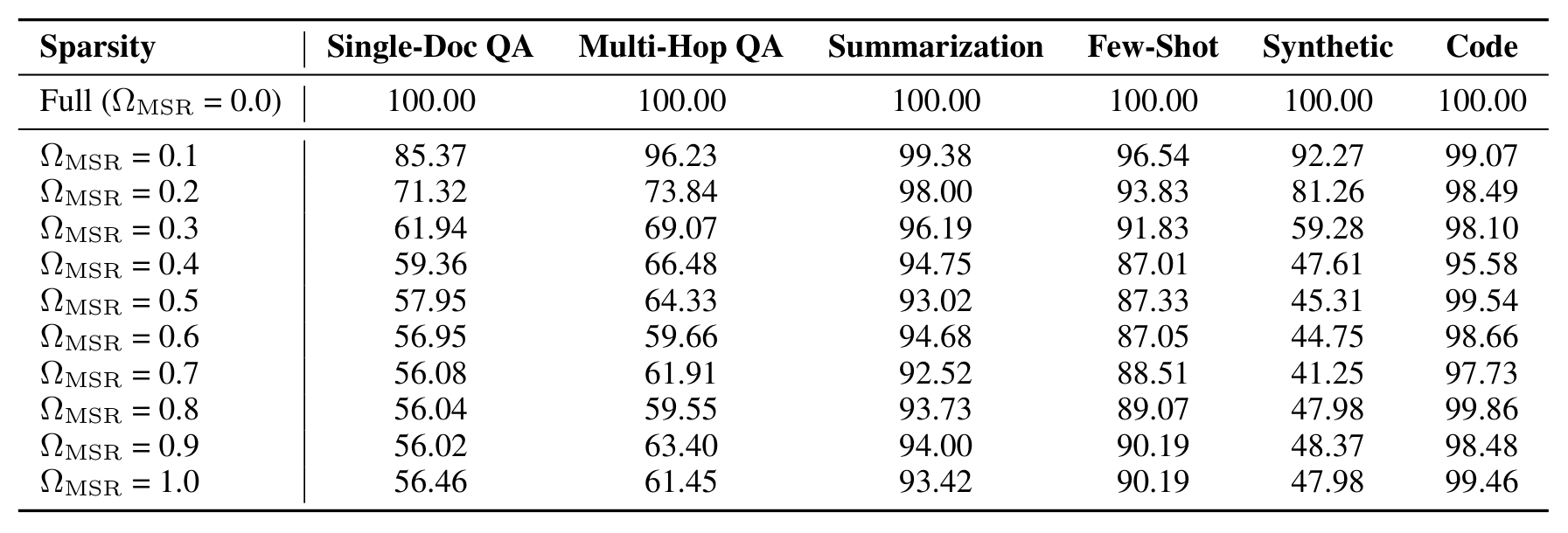
The motivating experiment: replace retrieval heads (ranked by the Retrieval Head method of Wu et al., 2024) with streaming-sparse heads one by one on Llama-3.1-8B-Instruct, and watch six task families.

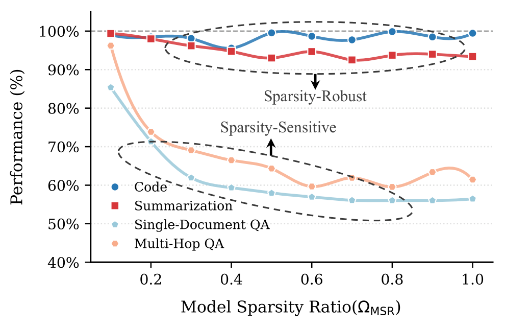
Table 7: retention rates across sparsity levels — **Table 7:**Performance retention rates across various model sparsity ratios. The values represent the percentage of performance relative to the Full Attention baseline (Sparsity 0.0), where 100.00 indicates parity. Rows denote the model sparsity ratio, and columns denote the evaluation tasks. Two worlds by column: Summarization keeps 92–99% from $\Omega_{\text{MSR}}$=0.1 all the way to 1.0, and Code stays ≥95% — coarse context suffices. Single-Doc QA drops to 85.4% already at 0.1 and 61.9% at 0.3; Multi-Hop QA and Synthetic collapse between 0.2–0.4. Tasks need only one bit of information — "does this input need fine-grained evidence?" — not a per-task sparsity configuration. Report p.15

Figure 2: performance trend as sparsity increases — **Figure 2:**Trend of model performance as the hybrid model sparsity ratio ($\Omega_{\text{MSR}}$) increases. We report model performance as a relative percentage score with respect to that of FA. The sparsity-robust family (blue) stays essentially flat even at $\Omega_{\text{MSR}}$=1.0; the sparsity-sensitive family (red) falls off early. The point where the curves fork is exactly why a single static ratio cannot serve both. Report p.2

Takeaway: tasks collapse into two regimes, so the routing decision is binary per head. Elastic Attention never has to learn per-task coefficients — just an input-conditioned on/off switch, placed at every KV head.

03 · Method

Method: the Attention Router

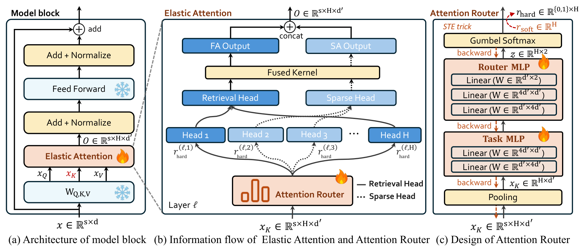
The recipe: keep the backbone frozen and bolt a small switchboard onto each layer's attention. Figure 3 shows the adapted block, the information flow, and the router itself.

Figure 3: Elastic Attention architecture — **Figure 3:**Illustration of our proposed Elastic Attention. (a) shows the adapted model block with frozen backbone parameters; (b) details the dynamic assignment of heads via the Attention Router module; (c) presents the lightweight design of the Attention Router. (a) the frozen backbone with the router attached; head outputs take the FA or SA path, concatenate, and pass through the fused kernel and FFN. (b) the router reads key hidden states $x_K$ and emits a binary decision $r$ per head — blue/red mark retrieval vs sparse heads, all executed inside one fused kernel. (c) pooling → Task MLP → Router MLP → Gumbel-Softmax → hard routing, with gradients flowing back through the straight-through estimator. Cost: 0.27M parameters per layer (head dim 128). Report p.3

The router pools the key hidden states $x_K\in\mathbb{R}^{s\times H\times d'}$ along the sequence dimension into a per-head task representation, then runs a Task MLP (to disentangle task features) followed by a Router MLP (to score each head), producing logits $z\in\mathbb{R}^{H\times2}$ and a hard decision $r^{(\ell,h)}_{\text{hard}}\in\{0,1\}$. One easily missed engineering detail: the pooling only keeps the first and last 100 tokens — system instructions live at the head of the context, the user query at the tail, and the long document body is mostly noise for task identification (verified in Appendix G.5).

Configuration in numbers [organized from Appendix C.1]: router input = 100 leading + 100 trailing tokens; Task/Router MLP hidden size = $4\times d'$ (default); router LR $5\times10^{-4}$, regularization LR $1\times10^{-3}$; sequence length 65,536, global batch 48, 300 steps — all inside a 12-hour run on 8×A800 with the backbone frozen. Parameter ledger [estimated]: at 0.27M per layer (paper's figure) a 32-layer model adds ~8.6M parameters — under 0.3% of a 4B/8B backbone, far cheaper than any retraining-based route.

Training uses hard routing (to match inference) and solves its two problems with continuous relaxation and a gradient bypass:

$$r^{(\ell,h)}_{\text{hard}} = \operatorname*{arg\,max}_{c \in \{0,1\}} r^{(h,c)}_{\text{soft}}, \qquad r^{(\ell,h)}_{\text{hard}} = r^{(\ell,h)}_{\text{hard}} + \left[ r^{(\ell,h)}_{\text{soft}} - \operatorname{detach}\!\left(r^{(\ell,h)}_{\text{soft}}\right) \right] \tag{6,7}$$

where $r_{\text{soft}}$ comes from Gumbel-Softmax (Jang et al., 2016) with annealing, and the bracket term is the straight-through estimator (Bengio et al., 2013). The objective couples language modeling with a sparsity penalty whose Lagrange multipliers $\lambda_1,\lambda_2$ are learned by gradient ascent:

$$\max_{\lambda_1,\lambda_2} \min \mathcal{L}_{\text{language}} + \lambda_1 \mathcal{L}_{\text{diff}} + \lambda_2 \mathcal{L}_{\text{diff}}^2, \qquad \mathcal{L}_{\text{diff}} = \Omega_{\text{MSR}}(f_\theta(X)) - t \tag{8}$$

The target $t$ is a non-tight constraint — a direction, not a quota: $t_{\text{rob}}=1.0$ for robust tasks, $t_{\text{sen}}=0.7$ for sensitive ones. Appendix E spells out the differentiable machinery (Gumbel-Sigmoid, temperature annealing $\tau(p)=\max(\tau_{\min},\tau_{\text{init}}e^{-rp})$, $r=0.6$).

Takeaway: the contribution is not a stronger sparse attention, but handing the mode choice to the input: discrete per-head switching, inference-aligned hard routing, and a soft constraint that lets tasks differentiate themselves.

04 · Deployment

Deployment: one fused kernel for mixed heads

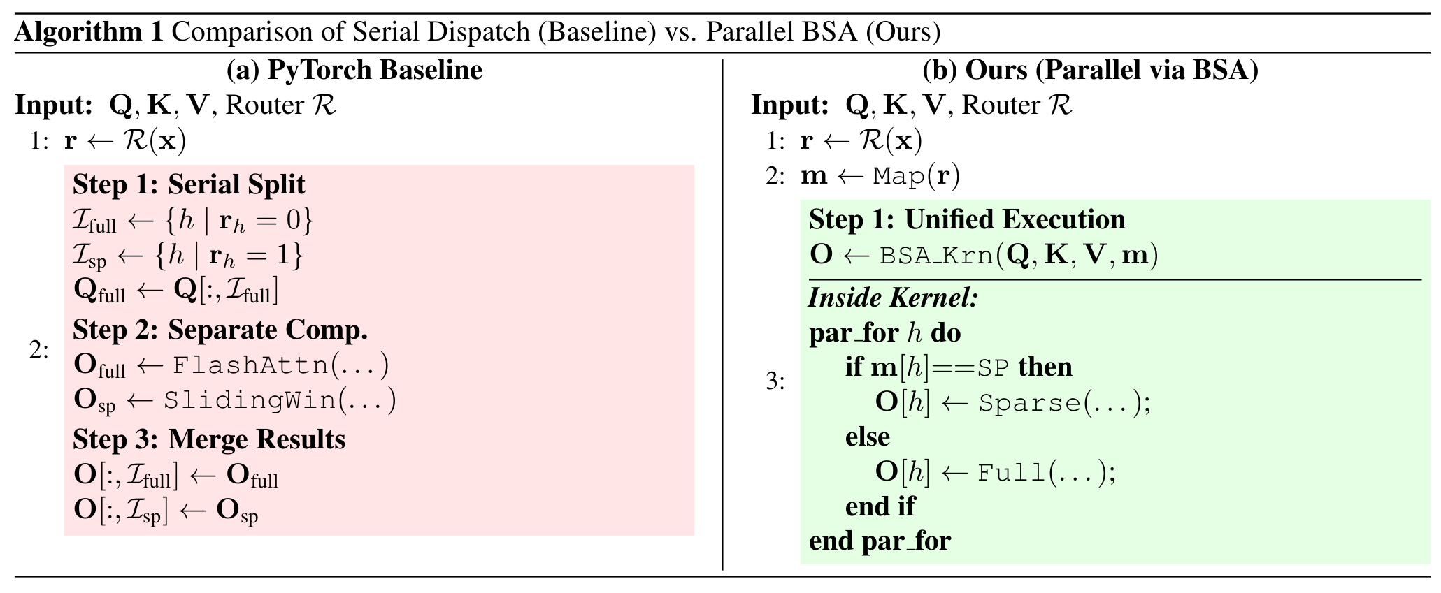
Mixed head types are a systems trap: the naive Serial Dispatch (Algorithm 1a) materializes split tensors, launches separate kernels, and fragments the sequence-dimension parallelism that long-context inference depends on. The paper's fix passes the routing decision as lightweight kernel metadata into a Block-Sparse-Attention kernel (Guo et al., 2024), so each thread block branches on its head's mode inside one launch.

Algorithm 1: serial dispatch vs parallel BSA — **Algorithm 1:**Comparison of Serial Dispatch (Baseline) vs. Parallel BSA (Ours). (a) the PyTorch baseline splits heads into $I_{\text{full}}$/$I_{\text{sp}}$ groups (explicit tensor copies, red), runs FlashAttention and sliding-window sparsity separately, then writes both outputs back. (b) the paper maps $r$ to metadata $m$, and the BSA kernel executes each head's branch in parallel with the grid (Batch × Heads × Sequence Blocks) left intact — no copies, no fragmentation. Report p.17

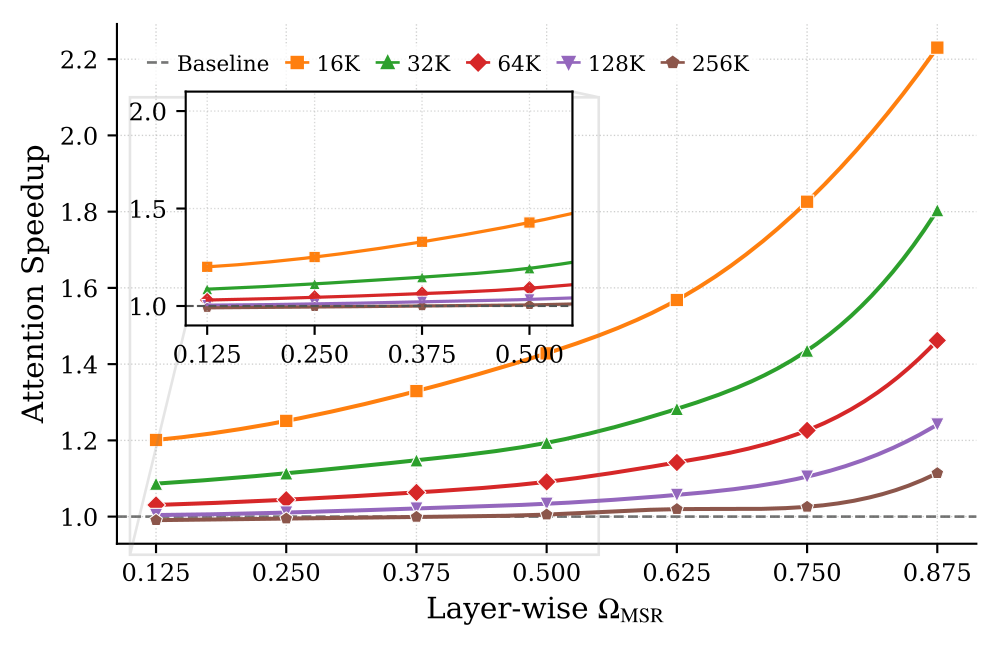
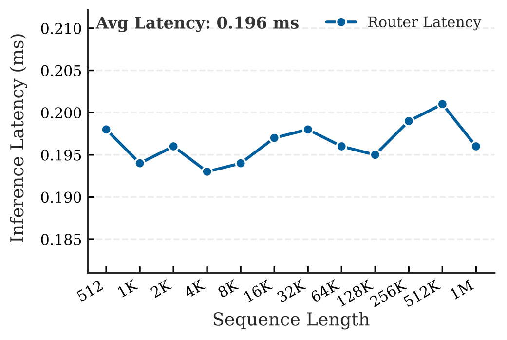
Figure 4: fused kernel speedup — **Figure 4:**Comparison of our fused kernel with a Torch-based sequential implementation for layer-wise hybrid attention. Speedup grows both with layer sparsity (0.125–0.875) and with sequence length (16K–256K), peaking around **2.2×**. Two readings: longer contexts benefit more (sequence-dimension parallelism is what fragmentation hurts), and sparser layers benefit more (more skipped SA work). Report p.4

Figure 10: router latency — **Figure 10:**Router latency analysis. The router incurs negligible overhead (avg. 0.196 ms). Our design ensures length-invariant stability, maintaining constant speed from 512 to 1M tokens. Avg. 0.196 ms and constant from 512 to 1M tokens — a direct payoff of boundary pooling: the router only ever reads 200 tokens, so its cost cannot grow with context. Report p.22

Scope (the paper is upfront): the design targets single-GPU or few-device deployment of small/medium models. Very large models are usually served with head-level parallelism across devices, which conflicts with layer-wise hybrid heads — the Impact Statement draws that boundary explicitly.

05 · Experiments

Experiments: three backbones, three suites

Setup [organized from §4.1 and Appendix C]: backbones Qwen3-4B, Qwen3-8B, Llama-3.1-8B-Instruct; training data blends five sources (ChatQA2-Long-SFT, MuSiQue, CoLT-132K, GovReport, XSum) into ~0.74B tokens spanning robust (code, summarization, in-context) and sensitive (single-/multi-doc QA) tasks at 8K–64K sequence length; targets $t_{\text{rob}}=1.0$, $t_{\text{sen}}=0.7$; 8×A800, under 12 hours per run. Baselines: DuoAttention, PruLong, InfLLM-V2 (training-based), MoBA, NSA, XAttention (other routes), all retrained in the same environment and evaluated through LOOM-Eval. Sparse-head implementations: SSA (streaming) and XA (XAttention), written as "{retrieval}-{sparse}", e.g. FA-SSA.

Main result ① — LongBench-E

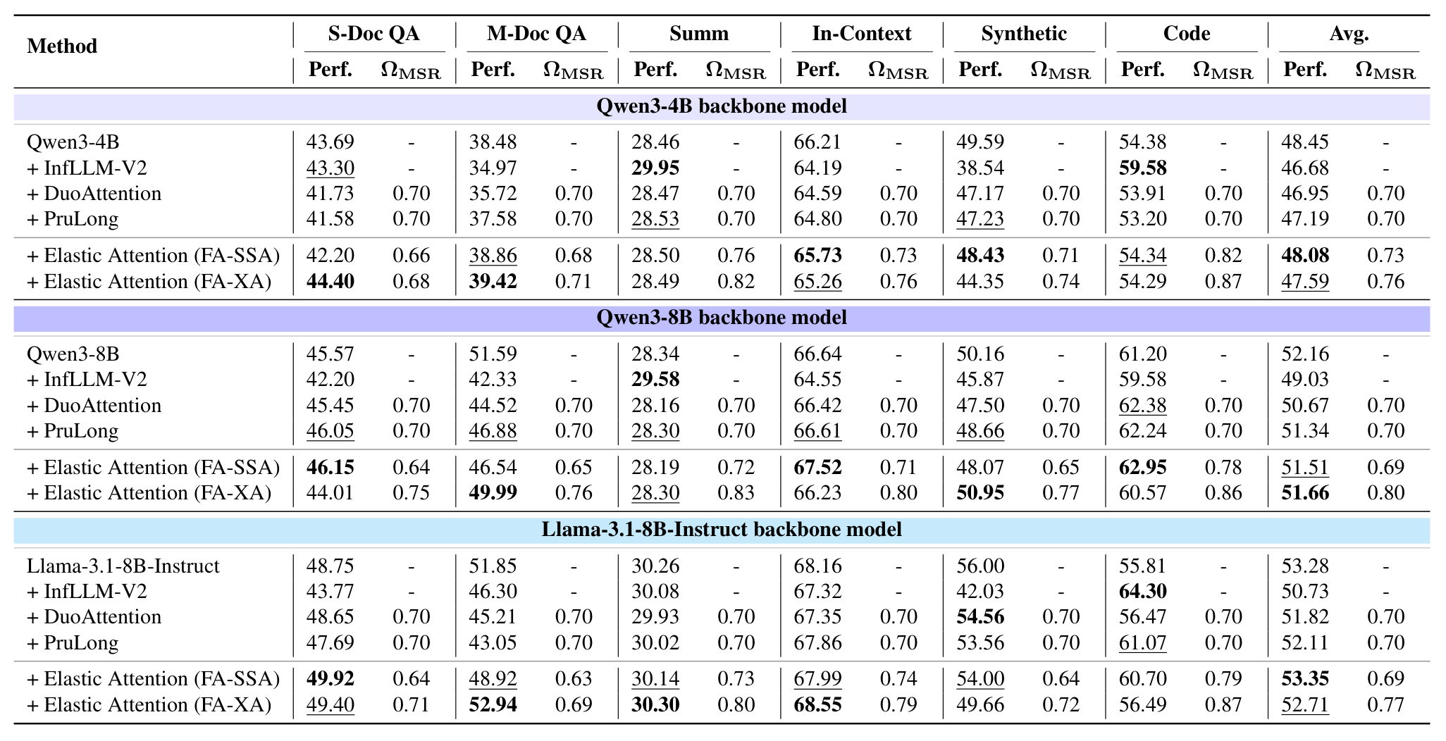
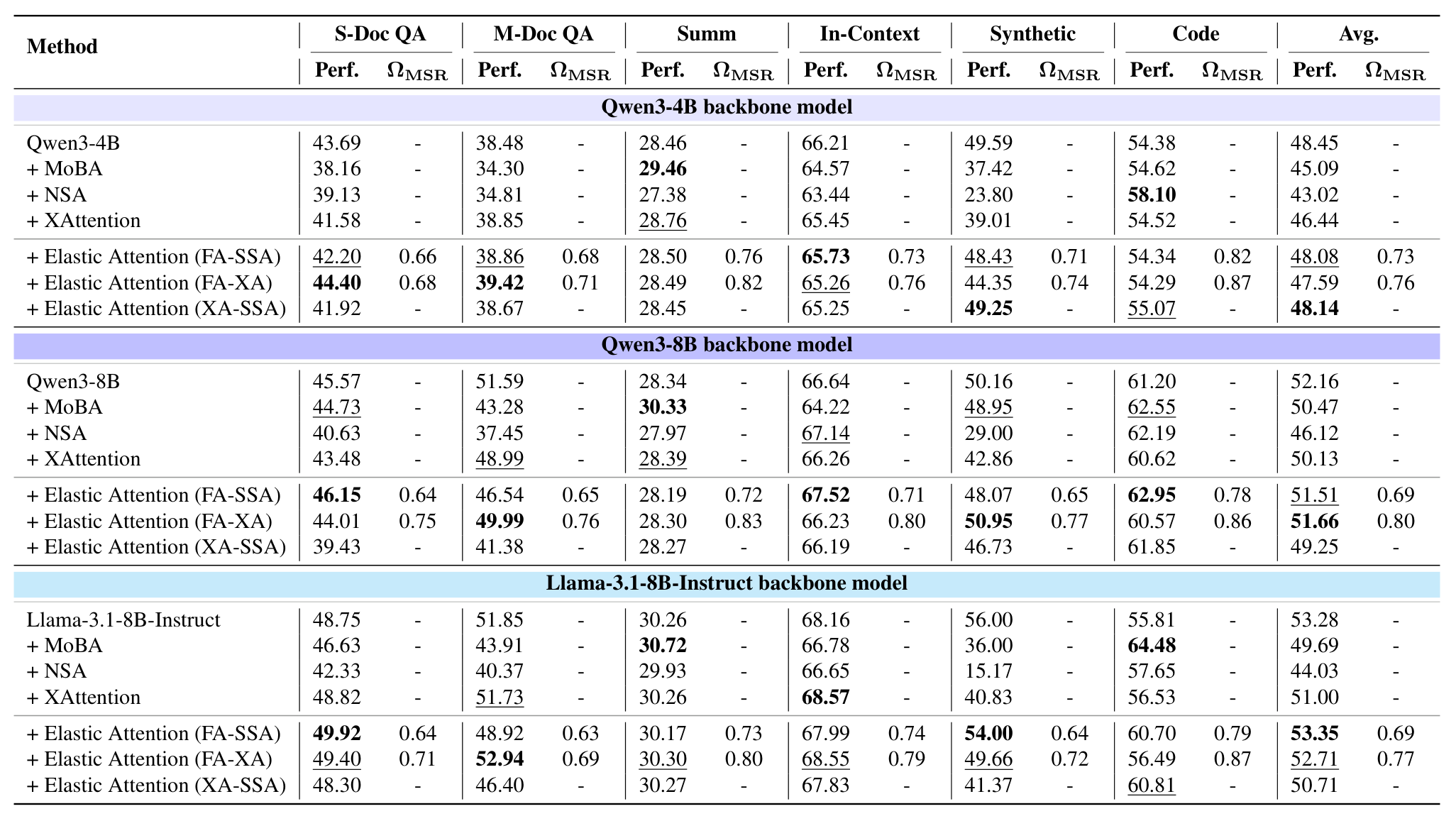
Table 1: LongBench-E main results — **Table 1:**Performance on LongBench-E (Bai et al., 2024). We report average performance (Perf.) and $\Omega_{\text{MSR}}$ per task category. The 1st and the 2nd performance in each comparison group are highlighted with bold font and underlined, respectively. Best average in all three groups: Qwen3-4B 48.08 (backbone 48.45, DuoAttention 46.95), Qwen3-8B 51.51 (52.16 / PruLong 51.34), Llama 53.35 (above the 53.28 backbone). The per-category $\Omega_{\text{MSR}}$ columns show the model spreading sparsity by task: code 0.78–0.82, summarization 0.72–0.73, QA 0.63–0.68 — no baseline does this (they are pinned at 0.70 or undefined). The paper notes that individual robust-task cells (Code/Summ) can favor baselines partly because Elastic Attention spends *less* compute there. Report p.5

Main result ② — RULER and LongBench-V2

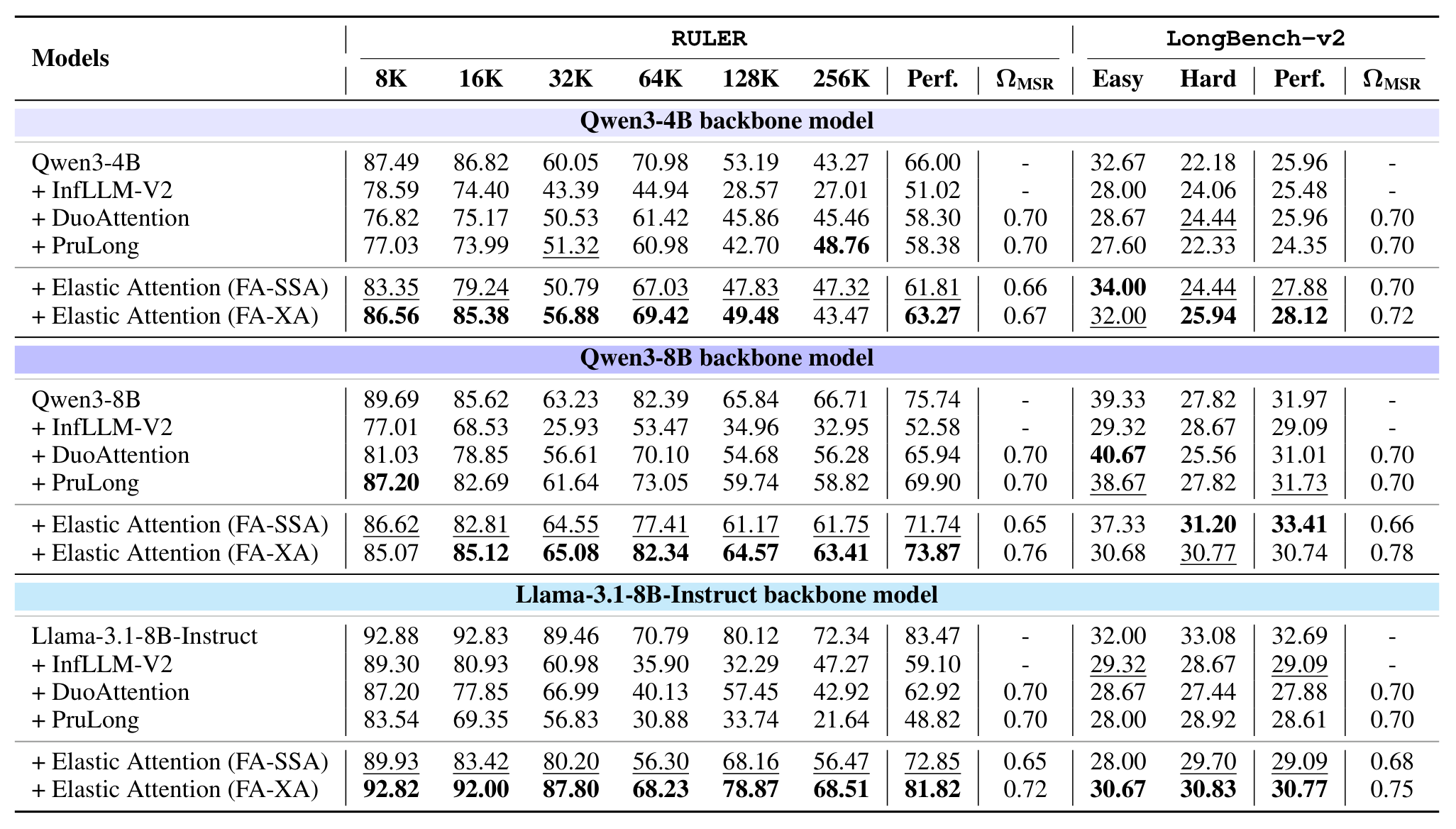
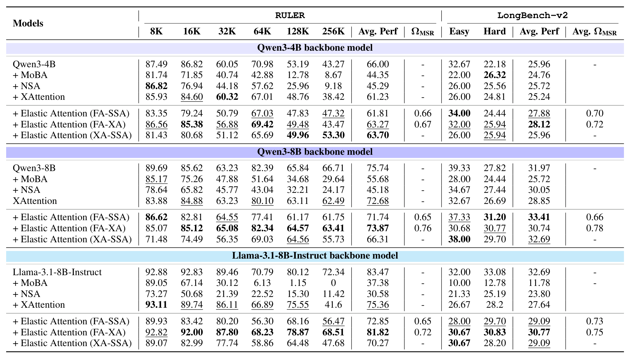
Table 2: RULER (8K–256K) and LongBench-V2 — **Table 2:**Model performance on RULER (Hsieh et al., 2024) and LongBench-v2 (Bai et al., 2025). We report the average Perf. and $\Omega_{\text{MSR}}$. Trained at 64K, evaluated to 256K. RULER averages: FA-XA reaches 63.27 / 73.87 / 81.82 against backbones 66.00 / 75.74 / 83.47, while DuoAttention manages only 58.30 / 65.94 / 62.92 and PruLong 58.38 / 69.90 / 48.82 — static ratios decay faster on extrapolation. On LongBench-V2, Elastic Attention beats the full-attention backbone on both Qwen backbones (27.88 / 33.41 vs 25.96 / 31.97). Beyond 64K at 8B scale, FA-XA wins because its lower $\Omega_{\text{ESR}}$ retains more effective information. Report p.6

Main result ③ — math reasoning and domain long documents

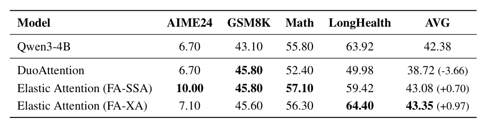
Table 3: AIME24 / GSM8K / Math / LongHealth — **Table 3:**Performance comparison across different benchmarks. The best results in each column are highlighted in bold. The values in parentheses indicate the performance gap relative to the Qwen3-4B baseline. On Qwen3-4B: FA-SSA wins all three math benchmarks (AIME24 6.70→10.00, GSM8K 43.10→45.80, Math 55.80→57.10); FA-XA tops LongHealth at 64.40. Averages: backbone 42.38, FA-SSA 43.08 (+0.70), FA-XA 43.35 (+0.97), DuoAttention 38.72 (−3.66). Moderate sparsity can act like regularization here — "sparse" does not automatically mean "worse". Report p.6

Efficiency and effective sparsity

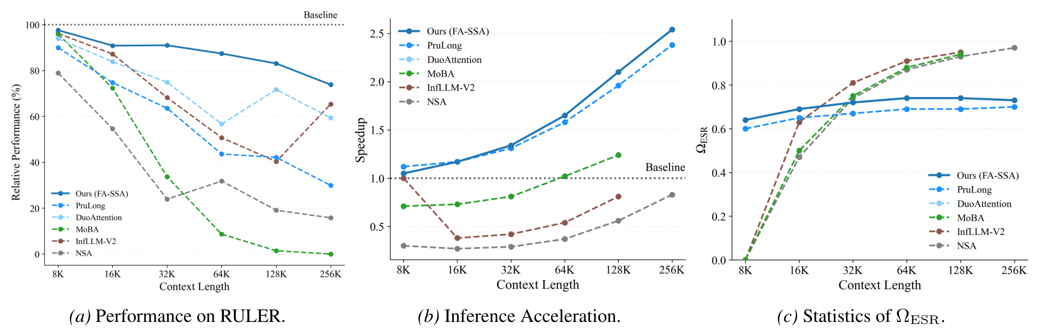
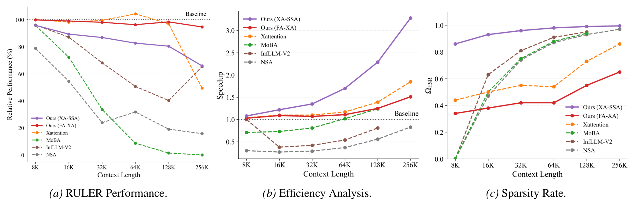
Figure 8: RULER performance, speedup, and Ω_ESR statistics — **Figure 8:**Comparison of performance and inference speedup on the RULER benchmark across different methods. We adopt Llama-3.1-8B-Instruct as the backbone model and compare with training-based methods (FA-SSA), as well as other cutting-edge sparse attention methods. We report $\Omega_{\text{ESR}}$, as it provides a fair comparison of the effective proportion of attended tokens across different approaches. (a) best performance across length buckets; (b) speedup keeps climbing with context because the model allocates higher sparsity to longer inputs; (c) $\Omega_{\text{ESR}}$ statistics — training-based hybrids hold a roughly constant effective sparsity, while Elastic Attention stays lower throughout. The paper also lists systematic failures of rivals: NSA/InfLLM-V2 require KV head counts divisible by 16, and MoBA/InfLLM-V2 reserve budget for sequence-level features, causing OOM at 256K. Report p.9

Scalability: the fully sparse regime and continued pretraining

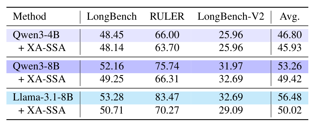
Table 5: XA-SSA fully sparse setting — **Table 5:**Results of implementing retrieval heads with XA. Making even retrieval heads sparse costs 0.87 points on Qwen3-4B (46.80→45.93, essentially free), but 3.8/6.5 points on Qwen3-8B and Llama (53.26→49.42, 56.48→50.02). That is the explicit accuracy-for-throughput trade at the extreme-efficiency end of the curve. Report p.8

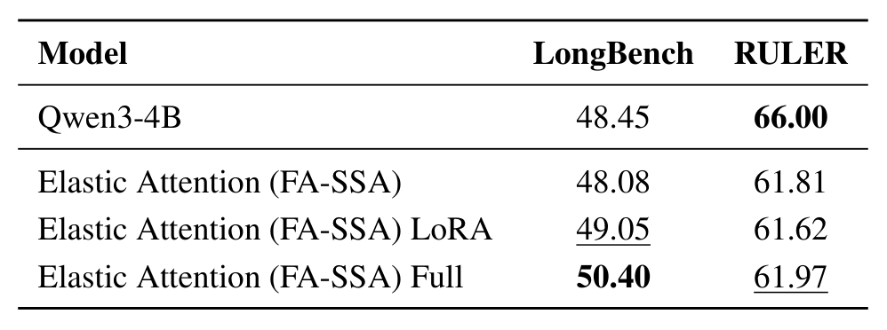
Table 6: frozen vs LoRA vs full fine-tuning — **Table 6:**Performance comparison of different tuning methods on LongBench and RULER. The best results are bolded, and the second-best are underlined. Relaxing the frozen-backbone constraint on Qwen3-4B: frozen 48.08 → LoRA 49.05 → full fine-tuning 50.40 on LongBench, while RULER stays flat (61.81 / 61.62 / 61.97). Elastic Attention composes with continued pretraining without sacrificing existing retrieval skills. Report p.8

Takeaway: same backbone, same data, same harness — best average on LongBench-E in all three groups, the largest margins in RULER's extrapolation range, and LongBench-V2 above the full-attention backbone, at the price of a 12-hour run and +0.27M params/layer.

06 · Analysis

Analysis: what the router learned

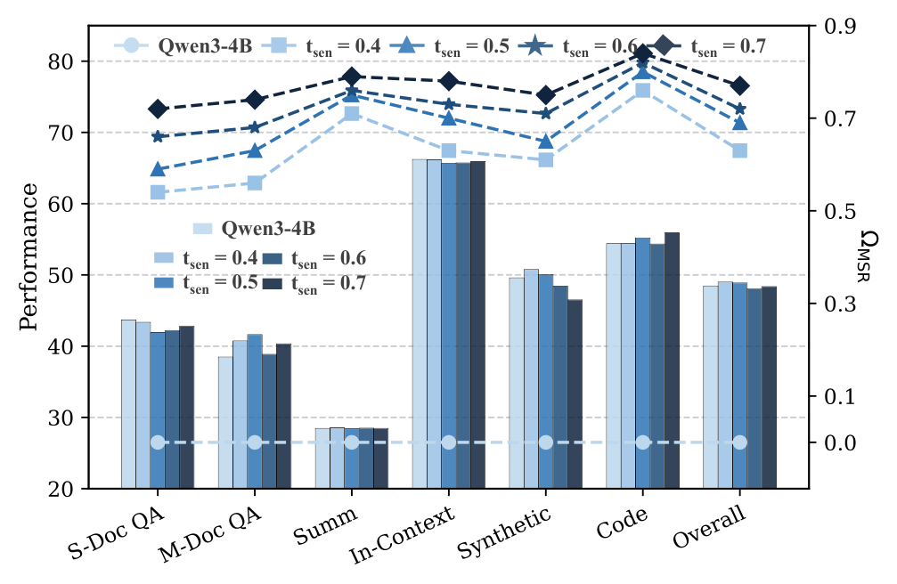
Figure 7: performance and Ω_MSR vs target sparsity t — **Figure 7:**Comparison of performance and test-time $\Omega_{\text{MSR}}$ among different training sparsity target $t$ settings. The bar chart denotes the performance and the line chart denotes $\Omega_{\text{MSR}}$ in each task. Lowering the sensitive-task target from 0.7 to 0.4 widens the gap between tasks and can even push performance past the backbone — yet the paper keeps $t_{\text{sen}}=0.7$, choosing inference efficiency over a few extra points. Note the realized $\Omega_{\text{MSR}}$ never exactly matches $t$: the constraint is a direction, not a quota. Report p.7

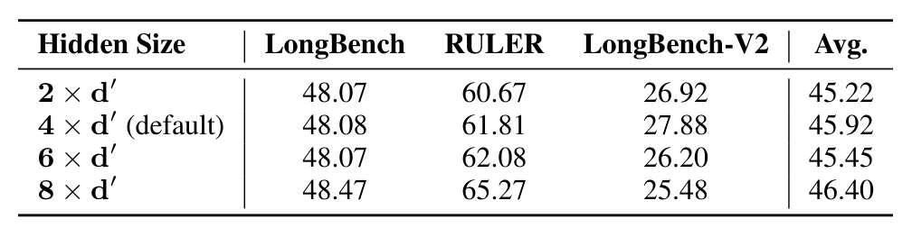
Table 4: MLP hidden dimension ablation — **Table 4:**Comparison among different MLP hidden dimensions. Average scores are nearly flat across $2\times$–$8\times d'$ (45.22 / 45.92 / 45.45 / 46.40); the paper keeps the default $4\times d'$ as the best trade-off. Routing power comes from the task-representation abstraction, not MLP capacity. Report p.7

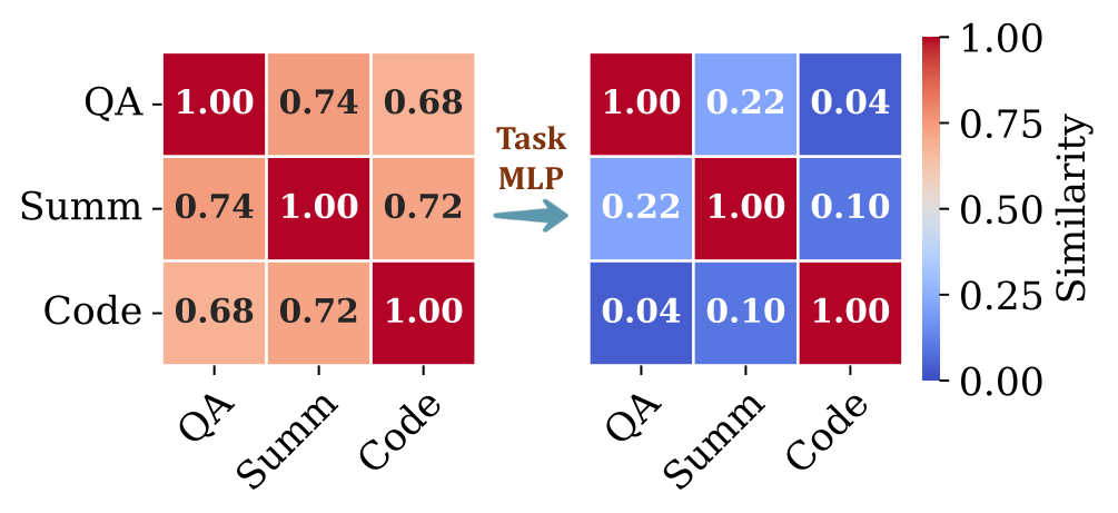
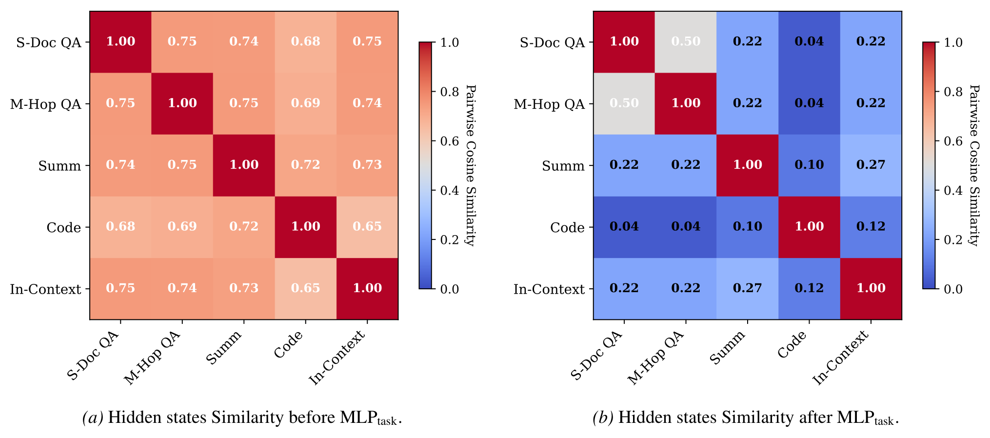
Figure 5: task representation similarity before/after Task MLP — **Figure 5:**Visualization of task representation similarity. (Left) before Task MLP, the pooled hidden states exhibit high pairwise cosine similarity across different tasks; (Right) after passing through the Task MLP, the inter-task similarity significantly decreases. Before the Task MLP, pooled hidden states look alike across tasks; afterwards they separate sharply. The Task MLP's job is exactly to disentangle task features for the Router MLP to act on. Report p.7

Figure 9: pairwise cosine similarity of routing representations — **Figure 9:**Pairwise cosine similarity of routing representations $z_{\text{task}}$. The prevalence of near-zero scores ($M_{uv}\approx 0$) indicates that the router maps distinct tasks to orthogonal subspaces on the local manifold. This confirms that the model implicitly disentangles task semantics into independent directions without supervision. 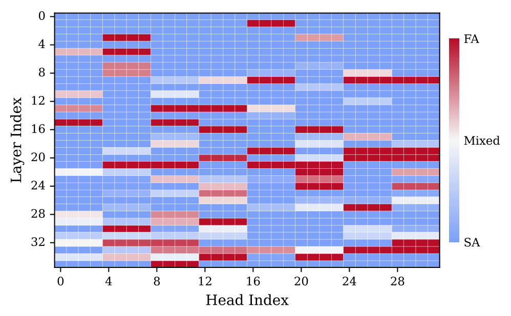With a stricter conditional-rescaling metric, most task pairs land near zero similarity — the router maps tasks to nearly orthogonal subspaces, entirely without task labels. The mechanism is a by-product of the sparsity-performance objective. Report p.22

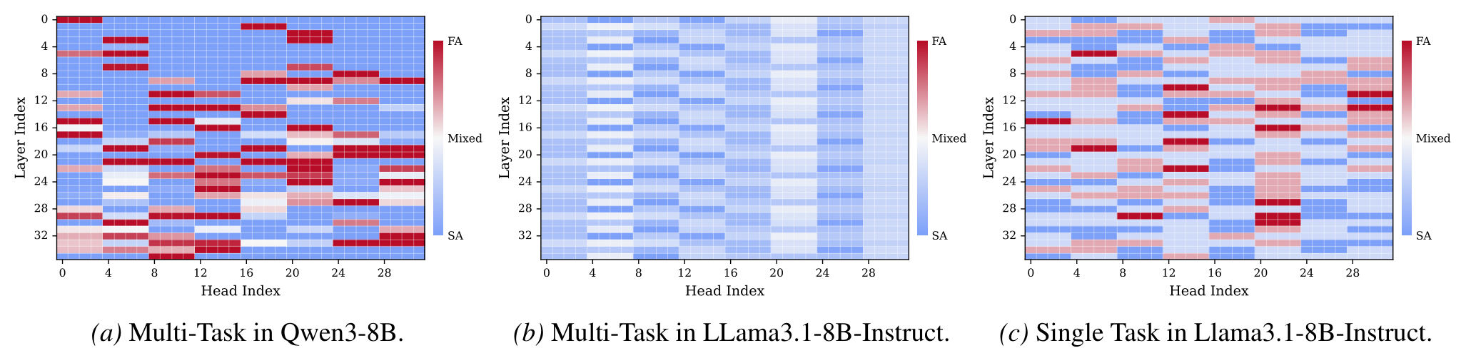
Figure 6: per-head routing activation frequency (Qwen3-4B) — **Figure 6:**Overview of routing activation frequency of each head in Qwen3-4B. Red indicates heads that are consistently routed to FA (i.e., retrieval heads) across all 6 tasks in LongBench-E, while blue denotes heads that are consistently routed to SA. A handful of heads — mostly in middle-to-upper layers — are consistently full attention, matching the retrieval-head literature; some heads switch with the task (light colors), and the rest stay sparse. Routing reproduces known model structure rather than adding noise. Report p.7

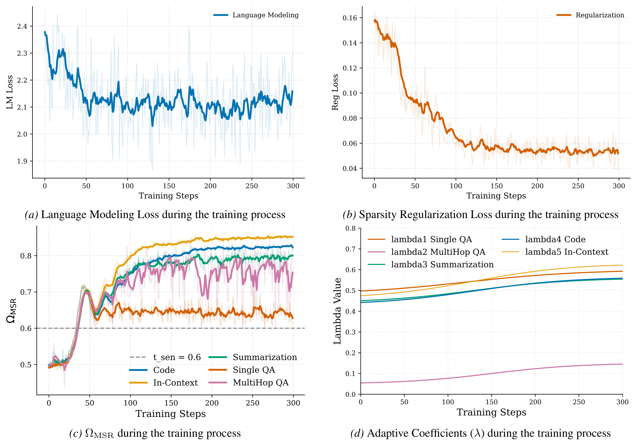
Figure 11: cross-model routing robustness — **Figure 11:**Extended Head Robustness Analysis. Similar to Figure 6, these heatmaps visualize the frequency of full-attention activation for each head. (a) and (b) show the multi-task global robustness for Qwen3-8B and Llama3.1-8B-Instruct, respectively. (c) presents the robustness analysis for Llama3.1-8B-Instruct in a single-task setting. Qwen3-8B shows task-agnostic structure (heads that are always active or always sparse); Llama-3.1 shows none in the aggregate view, yet its single-task breakdown reveals strong activations that migrate with the input. Qwen3 leans on fixed retrieval heads; Llama reallocates attention per task — the same router learns different policies per model family. Report p.22

Figure 13: training dynamics (LM loss / reg loss / Ω_MSR / λ) — **Figure 13:**Decomposition of Training Objectives for Elastic Attention. We visualize the training dynamics of the Attention Router, separating the total loss into (a) the primary language modeling objective and (b) the sparsity regularization term. Subfigures (c) and (d) illustrate the task-level differentiation in sparsity allocation ($\Omega_{\text{MSR}}$) and adaptive coefficients ($\lambda$), demonstrating how the model automatically distinguishes between sparsity-robust and sparsity-sensitive tasks. 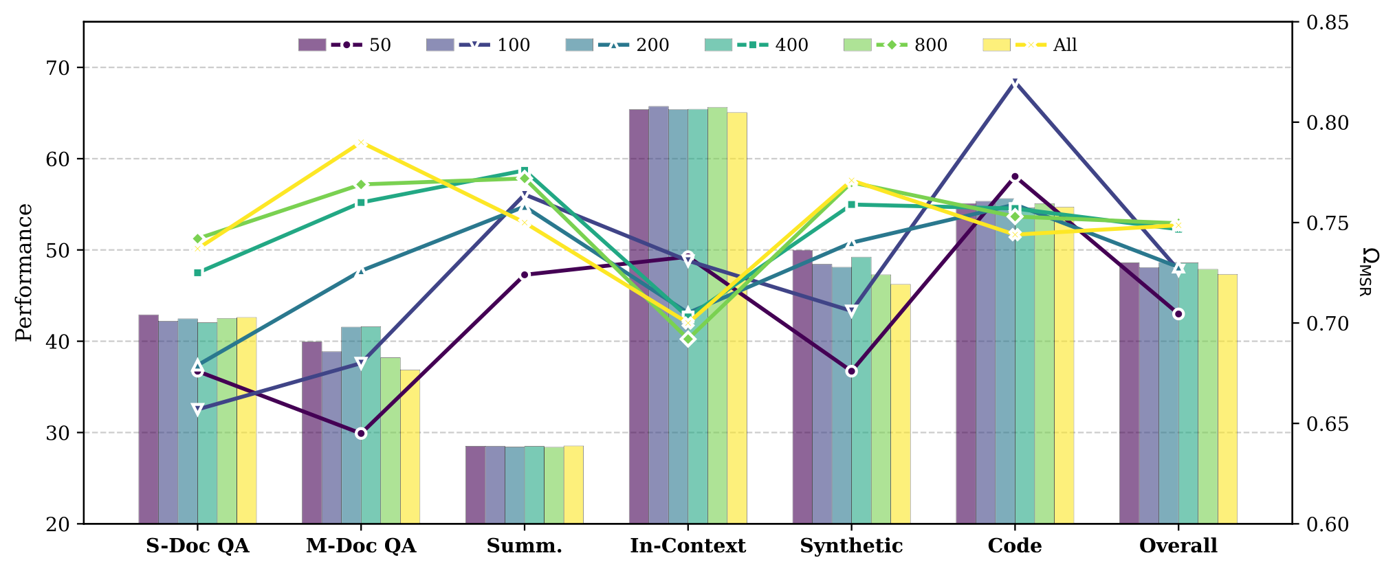(a) LM loss settles near 2.1 — sparsity injection does not disturb convergence; (b) the regularization loss falls from ~0.16 to ~0.06 within 100 steps; (c) per-task $\Omega_{\text{MSR}}$ diverges from a neutral start (code/in-context climb to ~0.80–0.85, QA plateaus near the target); (d) the Lagrange multipliers race — $\lambda_5$ (in-context) grows fastest, meaning the model prioritizes that task's density requirement. All within 300 stable steps. Report p.24

Figure 14: router input truncation — **Figure 14:**Impact of router input truncation length on downstream performance and $\Omega_{\text{MSR}}$. We compare varying truncation budgets ($L\in\{50,\dots,800,\text{All}\}$) applied to the concatenation of the sequence's prefix and suffix. Results indicate that increasing the input length beyond 100 tokens yields negligible performance gains and may degrade router selectivity due to a lower signal-to-noise ratio. Performance saturates at 100–200 tokens; longer inputs dilute the task signal (Multi-Doc QA actually degrades). This is the empirical basis for the 100+100 boundary-pooling default — and why router latency is length-invariant (Figure 10). Report p.25

Figure 12: length extrapolation and sparsity dynamics — **Figure 12:**Analysis of length extrapolation capability and sparsity dynamics on the RULER benchmark (8K-256K). We adopt Llama-3.1-8B-Instruct as the backbone model to compare our Elastic Attention variants (FA-XA and XA-SSA) with including MoBA and NSA. (a) at 256K, MoBA and NSA collapse toward zero while FA-XA holds 68.51 and XA-SSA 47.68 (far above the XAttention baseline's 35.82); (b)(c) NSA/InfLLM-V2 reach higher nominal sparsity (>0.95) but deliver under 1.0× speedup, whereas XA-SSA converts ~0.995 sparsity into a **3.28×** speedup and FA-XA trades at 1.51×. Two ends of a superior Pareto frontier. Report p.23

Takeaway: the Task MLP orthogonalizes task representations without supervision; routing rediscovers retrieval heads and even learns family-specific policies (fixed for Qwen3, migratory for Llama); sparsity differentiation emerges within 300 steps; and 200 tokens of routing input suffice. The model already contained a task-sensitivity structure — the router just reads it out.

07 · Appendix

Appendix: reproducibility, extra results, cases

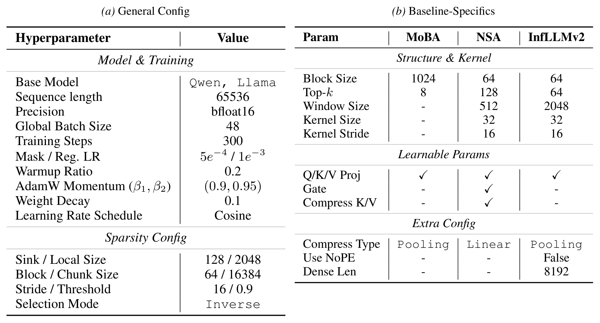
Table 8: hyperparameters — **Table 8:**Hyperparameters: General configuration (Left) and Baseline-specific settings (Right). Left: sequence 65,536, bfloat16, global batch 48, 300 steps, router/regularization LRs $5\times10^{-4}$/$1\times10^{-3}$, warmup 0.2, AdamW (0.9, 0.95), weight decay 0.1, cosine schedule; sparsity config sink/local 128/2048, block/chunk 64/16384, stride/threshold 16/0.9. Right: per-baseline block sizes (1024/64/64), top-k (8/128/64), windows (–/512/2048) — all retrained on the same data and environment. Report p.16

Table 11: RULER evaluation configuration — **Table 11:**Detailed configuration for the RULER benchmark evaluation. We evaluate across exponentially increasing context windows up to 256k tokens. RULER protocol: six lengths from 8K to 256K, 50 samples per task-length pair, NIAH retrieval family (single/multikey/multiquery/multivalue) plus QA extraction (qa1/qa2, fwe). Report p.20

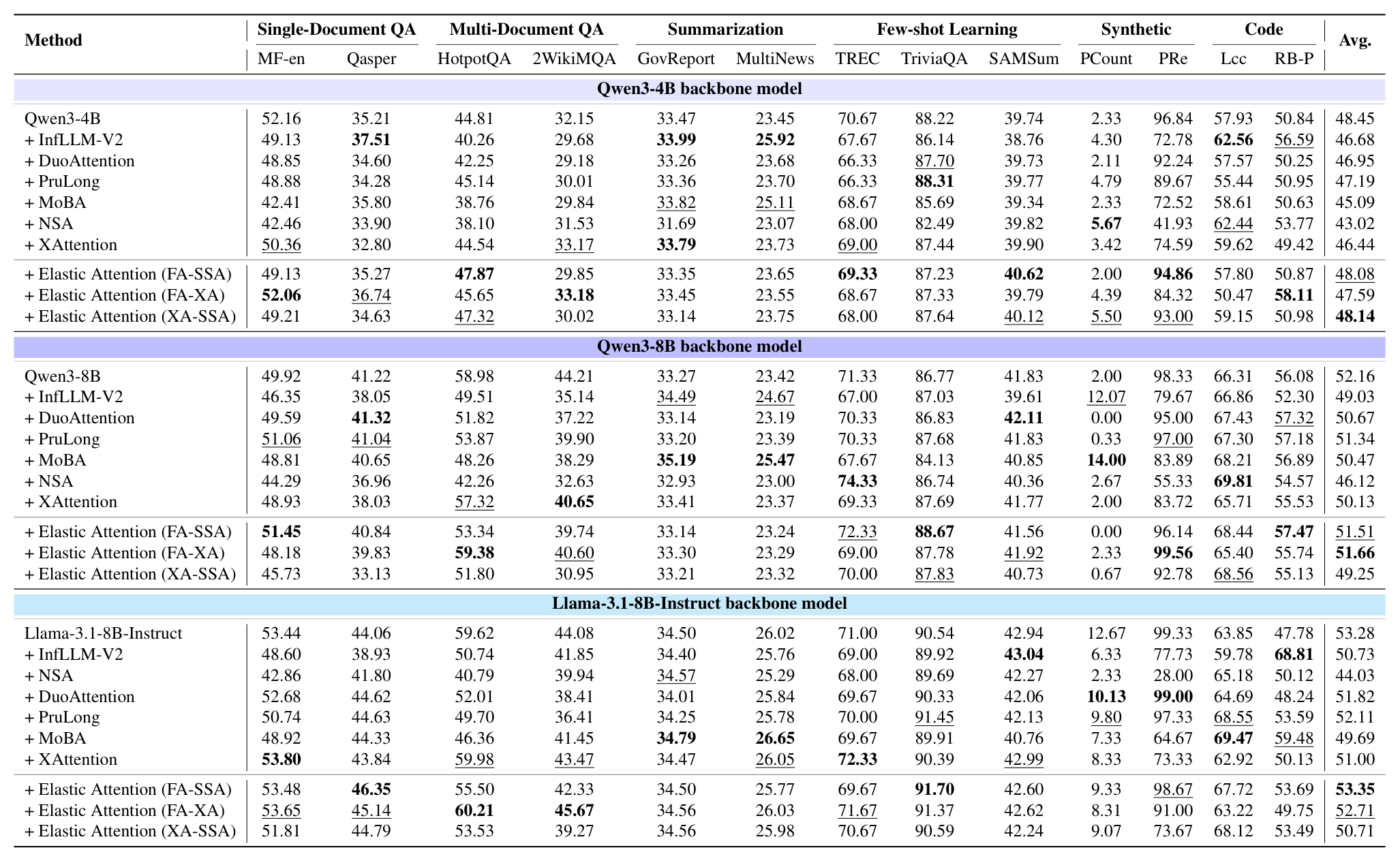
Table 9: full LongBench-E per-task results — **Table 9:**LongBench-E results comparison. The 1st and the 2nd performance in each comparison group are highlighted with bold font and underlined, respectively. All 13 sub-tasks (MF-en, Qasper, HotpotQA, 2WikiMQA, GovReport, MultiNews, TREC, TriviaQA, SAMSum, PCount, PRe, Lcc, RB-P) across the three backbone groups — the fine-grained companion to Table 1. Report p.18

Table 10: LongBench-E category averages with MoBA/NSA/XA-SSA — **Table 10:**Performance on LongBench-E. We report average performance (Perf.) and $\Omega_{\text{MSR}}$ per task category. The 1st and the 2nd performance in each comparison group are highlighted with bold font and underlined, respectively. The MoBA/NSA/XA-SSA-inclusive companion table. Elastic Attention's per-category $\Omega_{\text{MSR}}$ (e.g. QA 0.66–0.68 vs code 0.82 on Qwen3-4B) contrasts with baselines that are either pinned at 0.70 or undefined. Report p.19

Table 12: extra RULER / LongBench-V2 results — **Table 12:**Additional results on RULER and LongBench-v2. Per-length table including MoBA, NSA, XAttention. On Llama, MoBA dies from 32K (30.12 → 6.13 → 1.15 → 0) and NSA reaches only 11.42 at 256K, while FA-XA / XA-SSA hold 68.51 / 47.68 — the sharpest evidence that dynamic sparsity extrapolates better than static patterns. Report p.20

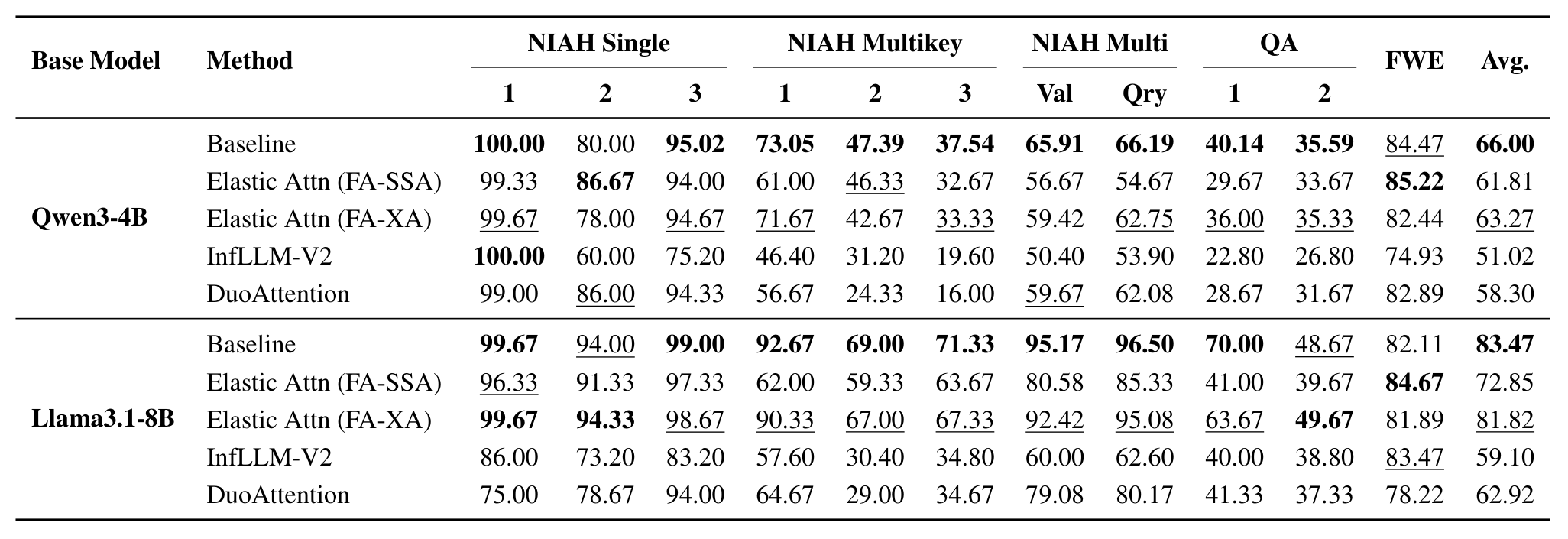
Table 13: RULER sub-task breakdown — **Table 13:**Performance comparison of different attention methods on RULER subtasks. Tasks are grouped logically to highlight performance variations. Sub-task detail (NIAH single/multikey/multi Val/Qry, QA1/QA2, FWE). On Llama, Elastic Attention (FA-XA) stays close to baseline on FWE (81.89 vs 82.11, where DuoAttention manages 78.22); the losses concentrate in the hardest multikey NIAH tiers. Report p.21

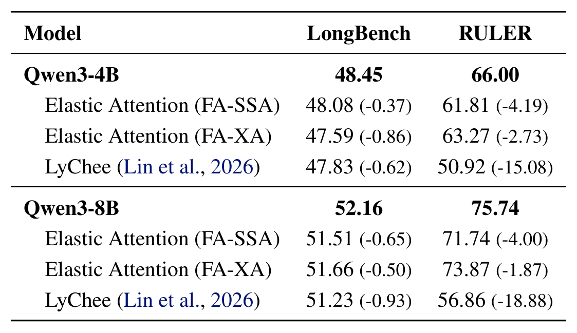
Table 14: comparison with LyChee — **Table 14:**Performance comparison on LongBench and RULER. The performance drop relative to the respective base model is shown in parentheses. Head-to-head with contemporaneous hybrid-head work LyChee: LongBench is close (−0.37 vs −0.62 at 4B; −0.65 vs −0.93 at 8B), but RULER separates them — Elastic loses 4.19/4.00 while LyChee loses **15.08/18.88**. Report p.21

Qualitative cases: three ways sparsity loses the detail

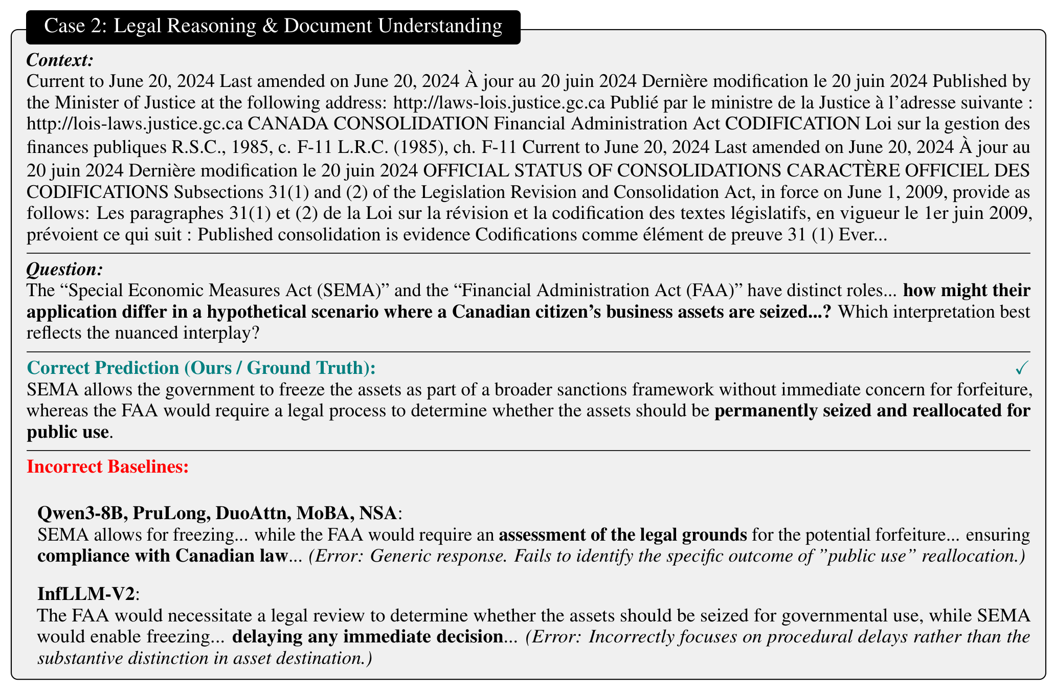
Figure 15: policy reasoning case — **Figure 15:**Qualitative comparison on a complex policy reasoning task. Our model correctly identifies the 'Gradual' approach required for stability, whereas baselines hallucinate 'Aggressive' or 'Immediate' measures that contradict the stability constraint. The question demands balancing fiscal sustainability, stability, and the energy transition. Elastic Attention picks the "gradual" package (green bank, subsidies kept five years, carbon tax deferred); baselines propose aggressive carbon taxes or immediate subsidy removal — fluent answers that violate the stated constraint. Report p.26

Figure 16: bilingual legal document case — **Figure 16:**Comparison on a bilingual legal document. Our model accurately extracts the specific legal provision regarding asset reallocation for public use (FAA), whereas baselines provide generic descriptions of “legal assessments” or “compliance” without specific details. SEMA vs FAA: the correct answer hinges on FAA's "reallocation for public use"; baselines answer with generic "legal review" boilerplate — sparse attention dropping the fine print and letting language priors fill it in. Report p.27

Figure 17: narrative entity tracking case — **Figure 17:**Qualitative comparison on narrative entity tracking. The task requires identifying the specific characters who conspired to frame the protagonist. Our model accurately retrieves the correct trio, whereas baselines consistently hallucinate “Villefort” (the public prosecutor) into the group, failing to distinguish between the plotters and the judicial figure involved later. Who wrote the incriminating letter in *The Count of Monte Cristo*? Correct: Danglars, Fernand, Caderousse. Several baselines add Villefort (who appears later) and InfLLM-V2 misses the mastermind entirely — exactly the entity relations sparsity tends to damage, and why sensitive tasks keep $\Omega_{\text{MSR}}$ at 0.63–0.68. Report p.28

Editor's note (paper typo): Appendix H says "In Table 15, 16, and 17, we present representative model outputs" — those numbers actually refer to Figures 15/16/17; no Tables 15–17 exist. Harmless, but recorded so readers don't hunt for missing tables.

08 · Commentary

Commentary

The paper's own conclusion and stated limits

Sorting tasks into robust/sensitive regimes and adding a per-head FA/SA router yields input-adaptive sparsity without touching the pretrained backbone — supported by three backbones and three suites, all trained in 12 hours. The authors explicitly bound the scope: ① the design targets single-GPU / few-device deployment of small-to-medium models (head-level parallelism on large clusters conflicts with layer-wise hybrid heads); ② sensitive tasks still trade accuracy for sparsity by scenario; ③ routing is decided once per request at the prefill stage.

Lineage and provenance (organized from the paper's citations)

Where each component comes from (organized from inline citations; not a table from the paper)
Component	Upstream as labeled by the paper	What this work changes
Retrieval heads	Retrieval Head (Wu et al., 2024)	Used to rank heads in the sparsity sweep (NIAH scoring + progressive replacement)
Hybrid-head mechanism	DuoAttention (Xiao et al., 2024a; 2025), PruLong (Bhaskar et al., 2025)	Static ratio → input-conditioned per-head routing
Sparse-head computation	Streaming Sparse Attention (Xiao et al., 2024b), XAttention (Xu et al., 2025)	Pluggable SA implementations (FA-SSA / FA-XA / XA-SSA)
Sparse kernel	Block-Sparse-Attention (Guo et al., 2024)	Routing decisions passed as kernel metadata; single launch for mixed heads
Routing mechanism	MoE gating (Shazeer et al., 2017)	"Choose an expert" → "choose an attention mode", per KV head
Relaxation & gradients	Gumbel-Softmax (Jang et al., 2016), STE (Bengio et al., 2013), reparameterization (Bhaskar et al., 2025)	Hard routing forward + soft gradients backward, with temperature annealing
Constrained optimization	Lagrangian multipliers (gradient ascent on $\lambda$)	Non-tight sparsity targets with bounds, letting tasks self-differentiate
Backbones	Qwen3 (Yang et al., 2025), Llama 3 (Grattafiori et al., 2024)	Three 4B/8B backbones, all frozen
Training data	ChatQA2 (Xu et al., 2024), MuSiQue (Trivedi et al., 2022), CoLT-132K (Li et al., 2025), GovReport (Huang et al., 2021), XSum (Narayan et al., 2018)	Blended into a ~0.74B-token dual-regime corpus
Evaluation & baselines	LOOM-Eval (Tang et al., 2025); DuoAttention / PruLong / InfLLM-V2 (Zhao et al., 2025) / MoBA (Lu et al., 2025a) / NSA (Yuan et al., 2025) / LyChee (Lin et al., 2026)	All baselines retrained in one environment, evaluated in one harness

Note: citations follow the paper's inline labels; this page does not verify each bibliography entry.

Not disclosed, worth testing next

Scale ceiling: validation stops at 4B/8B; larger dense models and MoE architectures are untested — MoE is itself a dynamic per-token compute regime, and the interaction is unexamined;
Context ceiling: RULER to 256K (trained at 64K); no 1M-scale extrapolation;
Decision granularity: one routing decision per request at prefill — per-turn or per-step re-routing (and its cost/benefit) is left open;
Evaluation breadth: three long-context suites only (no ∞Bench / multimodal long documents); the 0.74B-token training corpus is small, so the scaling curve of data is unknown;
Reproducibility details: code is released (LCM-Lab/Elastic-Attention) but the paper pins no commit or seed protocol.

Editor's commentary

A paper with a well-posed question. Most sparse-attention work optimizes which tokens to keep; this one steps back and asks whether to be sparse at all — a decision that varies with the input. The chain is clean: a two-regime observation, a binary per-head route, done.

The engineering closes the loop. Many dynamic schemes die on overhead: splitting tensors, launching kernels, fragmenting sequence parallelism. Passing routing as kernel metadata plus boundary-pooled routing (0.196 ms, length-invariant) makes the dynamism nearly free — and Figure 4 shows the fused kernel scaling to ~2.2×.

Cost is the headline. Twelve hours on 8×A800, frozen backbone, 0.27M params/layer — an architectural capability delivered at fine-tuning cost. For teams without large compute, that leverage is the most transferable lesson.

Reservations: ① "Elastic" is per-request, not per-token — a long chain-of-thought runs on one decision; ② the method does not solve token selection; it depends on the SA mechanism below it; ③ on Llama, FA-SSA still trails full attention by ~10 RULER points, and the fully sparse 8B variant degrades visibly — "approaching full attention" currently holds at the 4B scale and in sensitive-task regimes; ④ the orthogonality evidence is elegant, but the router likely captures only the task-type axis — whether it can exploit finer-grained input complexity is untested.

One line: Elastic Attention turns the sparsity ratio from a pre-deployment hyperparameter into a runtime variable — two task regimes observed, a 0.27M-param-per-layer router doing per-head binary routing, and a fused kernel that makes dynamism cheap. Twelve hours of training buys a cost-quality curve that stretches with the input.

Glossary

Reading glossary

Abbreviations used above (dotted-underlined terms in the prose show tooltips too).

Reading glossary (dotted-underlined abbreviations in the prose show hover definitions)
Term	Full name	One-line explanation
FA	Full Attention	Every token attends to all previous tokens — accuracy ceiling, cost ceiling
SA	Sparse Attention	Only a fraction of K/V is computed — cheaper but can drop detail
Ω_MSR	Model Sparsity Ratio	Share of KV heads assigned to SA (Definition 2.1)
Ω_ESR	Effective Sparsity Ratio	Sparsity weighted by each head's pruning rate ρ (Definition 2.2)
SSA	Streaming Sparse Attention	Attention-sink + sliding-window pattern (Xiao et al., 2024b)
XA	XAttention	Training-free block-sparse attention using antidiagonal scoring (Xu et al., 2025)
BSA	Block-Sparse-Attention	Kernel used here to execute mixed heads in one launch (Guo et al., 2024)
STE	Straight-Through Estimator	Hard values forward, soft gradients backward
DuoAttention / PruLong / InfLLM-V2	—	Training-based hybrid/KV-pruning baselines retrained in this paper
MoBA / NSA	Mixture of Block Attention / Native Sparse Attention	Representative sparse-attention architectures used as baselines
NIAH	Needle-in-a-Haystack	The classic long-context retrieval probe, RULER's main task family
RULER	—	Configurable synthetic long-context benchmark (Hsieh et al., 2024)
LongBench-E / -V2	—	Real-world long-context suites (14 tasks; and the 8K–2M-word reasoning upgrade)
FWE	Fuzzy Word Extraction	RULER's fine-grained extraction sub-task
LOOM-Eval	—	Long-context evaluation framework used here (Tang et al., 2025)
LyChee	—	Contemporaneous hybrid-head sparse decoding work (Lin et al., 2026)