论文精读 · Elastic Attention:测试时自适应稀疏比的 Transformer 高效推理

01 · Overview

速览:一页看懂 Elastic Attention

长上下文推理的成本大头在注意力。业界的主流解法是混合注意力:一部分头做全注意力(FA)保精度,另一部分头做稀疏注意力(SA)省算力。但"FA 占多少"这个比例通常是拍定的静态值——而论文的初步实验显示(见 §3),不同任务对稀疏的敏感度完全不同:摘要、代码这类任务可以稀疏到极致,而问答类任务一旦越过阈值就断崖式下跌。既然如此,模型为什么不在推理时自己决定这一次要多稀疏?

读数约定:本页全部数字以论文原文为准;凡由本页依据论文配置整理、归纳或换算的内容,均以「整理」「推算」显式标注,便于与论文口径区分。记号沿用论文:FA=全注意力,SA=稀疏注意力,$\Omega_{\text{MSR}}$=模型稀疏比(稀疏头占比),$\Omega_{\text{ESR}}$=有效稀疏比(计入每个头的剪枝率),$t$=训练时的目标稀疏比。

训练预算

12 小时 · 8×A800骨干完全冻结,只训练 Attention Router

Router 开销

+0.27M 参数/层头维 128 假设;平均延迟 0.196 ms

训练数据

0.74B tokens8K–64K 序列,5 个数据源

测试时稀疏比

$\Omega_{\text{MSR}}$ 0.63–0.85按任务自适应:代码 ~0.82、QA ~0.63–0.68

推理加速

1.51× – 3.28×FA-XA / XA-SSA,RULER 256K

评测规模

3 骨干 × 3 长上下文基准Qwen3-4B/8B、Llama-3.1-8B-Instruct

论文的开篇图把"动态稀疏"的收益摆上台面——同一个模型,两种设置,和既有稀疏注意力方法同场比较:

Figure 1: Elastic Attention 与既有方法在 LongBench-V2 上的对比 — **Figure 1:**Comparison between Elastic Attention (ours) and existing approaches on LongBench-V2 (Bai et al., 2025). “(XA+SSA)” and “(FA+SSA)” denote our different settings. LongBench-V2 上的总览对比。两种设置的含义:FA-SSA = 保留检索头做全注意力、其余头走流式稀疏;XA-SSA = 连"检索头"也用 XAttention 这种训练无关的块稀疏方法实现,整模型进入全稀疏区间——前者守精度,后者拼效率。图中横轴与纵轴的精确口径见原文;后面 Figure 8 与 Table 2 给出逐长度的读数。论文特意在正文提醒:NSA、InfLLM-V2 这类方法对 KV 头数有架构约束(如必须为 16 的倍数),与 Llama-3.1-8B 等模型的头数并不兼容,而 Elastic Attention 不改变骨干结构。报告 p.1

💡 点击任意图片可查看原始高清大图,再次点击或按 Esc 关闭。

小结:Elastic Attention 的三个动作——①观察:把下游任务归成"稀疏鲁棒"与"稀疏敏感"两类(§3);②路由:轻量 Attention Router 按输入把每个 KV 头分到 FA/SA,用 Gumbel-Softmax + STE 训练(§4);③落地:融合 kernel 让同一层里不同模式的头在一次前向里并行算完(§5)。三者合起来,把"静态比例"换成了"每次推理现算的比例"。

02 · Background

背景:FA、SA 与混合头机制

标准全注意力(FA)的计算量与上下文长度的平方成正比,这是长上下文推理的第一成本项;稀疏注意力(SA)只保留最相关的一小部分 K/V(例如 20%),把成本压下来,但会牺牲精度。近年的折中方案是混合头机制:同一个模型里,一部分头做检索(走 FA),其余头走 SA。论文先把这个框架写成公式。

检索头与稀疏头

检索头(retrieval head)负责把上下文里真正相关的 token 找回来——长上下文能力的关键,通常用 FA 计算:

$$O_r = \mathrm{Softmax}\!\left(QK^{\top}\right)V \tag{1}$$

稀疏头则只保留一部分 K/V(记作 $\tilde{K},\tilde{V}$),用 SA 计算:

$$O_s = \mathrm{Softmax}\!\left(Q\tilde{K}^{\top}\right)\tilde{V} \tag{2}$$

混合头机制给第 $\ell$ 层第 $h$ 个 KV 头静态分配一个计算类型 $\pi(\ell,h)\in\{\text{FA},\text{SA}\}$,层输出按头拼接:

$$O^{(\ell)} = \mathrm{Concat}\!\left(O^{(\ell,1)}, O^{(\ell,2)}, \dots, O^{(\ell,H)}\right), \qquad O^{(\ell,h)} = \begin{cases} O_r, & \pi(\ell,h)=\text{FA} \\ O_s, & \pi(\ell,h)=\text{SA} \end{cases} \tag{3}$$

两个稀疏比指标

论文定义了贯穿全文的两个度量——这是读后续所有表格的钥匙:

$$\Omega_{\text{MSR}}(f_\theta) = \frac{1}{H}\frac{1}{L}\sum_{h=1}^{H}\sum_{\ell=1}^{L}\mathbb{I}\!\left[\pi(\ell,h)=\text{SA}\right] \tag{4}$$

$$\Omega_{\text{ESR}}(f_\theta) = \frac{1}{H}\frac{1}{L}\sum_{h=1}^{H}\sum_{\ell=1}^{L}\rho(\ell,h) \tag{5}$$

$\Omega_{\text{MSR}}$ 数的是"有多少头是稀疏头";$\Omega_{\text{ESR}}$ 则把每个头实际的剪枝率 $\rho$ 也算进去(FA 头 $\rho=0$;SA 头 $\rho=\rho_{\text{SA}}$,例如只保留 10% token 时 $\rho_{\text{SA}}=0.9$)。区分这两个指标很重要:加 1 个稀疏头的增益是台阶式的($1/(LH)$),省 token 的增益是连续的——后面 Figure 8(c) 用 $\Omega_{\text{ESR}}$ 做公平横轴,就是因为不同方法的稀疏粒度不同,只比 $\Omega_{\text{MSR}}$ 会失真。

为什么静态比例不够:混合头的比例是在推理前定死的。但论文的初步实验(§3)表明,不同任务对稀疏的容忍度差了一个量级——用一个固定比例服务所有请求,要么在敏感任务上掉分,要么在鲁棒任务上浪费算力。更麻烦的是:找一个"合适的比例"通常需要对每个任务做大量验证,工程上不可扩展。

03 · Observation

观察:任务天然分成两类

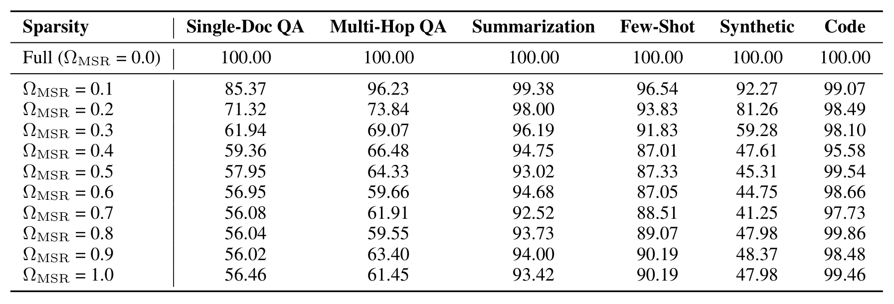
论文的出发点是一次系统的"稀疏扫描"实验:在 Llama-3.1-8B-Instruct 上按检索头排名(依据 Retrieval Head 方法,Wu et al., 2024)逐个把检索头替换成流式稀疏头,观察 6 类下游任务的表现如何随 $\Omega_{\text{MSR}}$ 变化。结果如下——这张表是全文最重要的动机证据:

Table 7: 不同稀疏比下各任务相对全注意力的保留率 — **Table 7:**Performance retention rates across various model sparsity ratios. The values represent the percentage of performance relative to the Full Attention baseline (Sparsity 0.0), where 100.00 indicates parity. Rows denote the model sparsity ratio, and columns denote the evaluation tasks. 按列读,任务的"抗稀疏"能力分成两个世界:**摘要(Summarization)**从 $\Omega_{\text{MSR}}$=0.1 到 1.0 始终保留 92%–99%,**代码(Code)**始终 ≥95%——这两类任务只需要粗粒度上下文,稀疏几乎无代价;**单文档 QA** 在 0.1 就掉到 85.4%,0.3 只剩 61.9%;**多跳 QA** 与 **Synthetic** 同样在 0.2–0.4 之间断崖。这就是"稀疏鲁棒 vs 稀疏敏感"两分法的直接证据:与其给每个任务学一个专属配置,模型只需要判断"这次要不要精细信息",二选一即可。报告 p.15

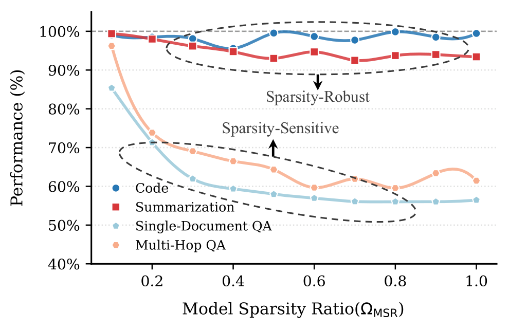
把同一批数据画成曲线,两个任务家族的形状差异一目了然:

Figure 2: 模型性能随混合稀疏比的变化趋势 — **Figure 2:**Trend of model performance as the hybrid model sparsity ratio ($\Omega_{\text{MSR}}$) increases. We report model performance as a relative percentage score with respect to that of FA. 蓝线族(稀疏鲁棒,如摘要)几乎水平:稀疏比一路加到 1.0,性能基本不动;红线族(稀疏敏感,如各类 QA)在中低稀疏比处就明显下坠。横轴的 $\Omega_{\text{MSR}}$ 从 0 到 1,相当于把全注意力模型逐步"抽稀"成纯稀疏模型——两条曲线的分叉位置,就是静态比例注定二选一的根源。报告 p.2

小结:观察的结论可以压缩成一句话——任务只分两类,路由只需二分。这为后面的方法定了形:不需要为每个任务学一套系数,只需要一个输入相关的二值决策(每个头 FA 还是 SA)。理论上,模型只要"判断这次输入是鲁棒型还是敏感型",就能把稀疏比放到合适的位置。

04 · Method

方法:Attention Router 与弹性路由

整体架构可以一句话概括:骨干不动,给每层的注意力加一个"开关面板"。Figure 3 把三件事画在一起:改造后的模型块、弹性注意力的信息流、以及路由器自身的结构。

Figure 3: Elastic Attention 总体架构(模型块 / 信息流 / Router 结构) — **Figure 3:**Illustration of our proposed Elastic Attention. (a) shows the adapted model block with frozen backbone parameters; (b) details the dynamic assignment of heads via the Attention Router module; (c) presents the lightweight design of the Attention Router. (a) 模型块:冻结的骨干参数旁挂上 Attention Router,头的输出经 Fa/SA 两条路径后拼接,再进 Fused Kernel 与 FFN;(b) 信息流:Router 读取 Key 隐状态 $x_K$,为每个头产出二值决策 $r$,蓝色/红色分别代表检索头(FA)与稀疏头(SA),所有头在同一个 fused kernel 里执行;(c) Router 结构:池化 → 两段 MLP(Task MLP 先推断任务特征,Router MLP 再逐头定模式)→ Gumbel Softmax → 硬路由,梯度经 STE 回传。整个 Router 只占 0.27M 参数/层(头维 128 假设下)。报告 p.3

Router 怎么工作

路由器的输入是 Key 的隐状态 $x_K \in \mathbb{R}^{s \times H \times d'}$($s$ 为序列长,$H$ 为 KV 头数,$d'$ 为头维)。它先沿序列维做池化,得到每个头的任务表征 $x'_K \in \mathbb{R}^{H \times d'}$;再依次经过 Task MLP(把任务特征从隐状态里"提纯")与 Router MLP(逐头打分),产出 logit 矩阵 $z \in \mathbb{R}^{H \times 2}$,经 softmax 分类器变成每个头的硬决策 $r^{(\ell,h)}_{\text{hard}} \in \{0,1\}$($0$=FA,$1$=SA)。

一个容易被忽略但很关键的工程细节:池化只取序列的首尾各 100 个 token(边界池化)。理由是系统提示词在开头、用户问题在结尾,中间的长文档对"判断任务类型"而言基本是噪声——论文在附录 G.5 用截断实验验证了这一点(见 §7)。

配置落到具体数字(据论文附录 C.1 整理):路由输入 = 首 100 + 末 100 token;Task/Router MLP 的中间隐维 = $4\times d'$(默认,$d'$ 为头维,即 128 → 隐维 512);Router 学习率 $5\times10^{-4}$、稀疏正则系数学习率 $1\times10^{-3}$;训练序列长 65,536、全局批 48、共 300 步。整套训练在 8×A800 上 12 小时内跑完,骨干参数全程冻结。
参数量这么算(本页推算):每层 +0.27M(论文口径),按 32 层模型约为 8.6M 的额外参数——相对 4B/8B 骨干不到 0.3%;代价远小于任何"重训骨干"的方案。

训练:硬路由 + 连续松弛

推理时用的是硬决策,为了不让训练和推理脱节,训练时也用硬路由——但这带来两个问题:softmax 分布怎么逼近硬决策?argmax 不可导怎么办?论文的两件工具都在公式里:

$$r^{(\ell,h)}_{\text{hard}} = \operatorname*{arg\,max}_{c \in \{0,1\}} r^{(h,c)}_{\text{soft}}, \qquad \forall h \in \{1, \dots, H\} \tag{6}$$

其中 $r^{(\ell)}_{\text{soft}} \in \mathbb{R}^{H \times 2}$ 由 Gumbel-Softmax(Jang et al., 2016)产生;argmax 不可导的问题用STE(Bengio et al., 2013)解决——前向保持硬决策,反向把梯度直接传给软分布:

$$r^{(\ell,h)}_{\text{hard}} = r^{(\ell,h)}_{\text{hard}} + \left[ r^{(\ell,h)}_{\text{soft}} - \operatorname{detach}\!\left(r^{(\ell,h)}_{\text{soft}}\right) \right] \tag{7}$$

训练目标则是一个带拉格朗日乘子的 min-max 形式:语言建模损失照常最小化,稀疏正则项负责把实际稀疏比 $\Omega_{\text{MSR}}$ 拉向目标 $t$,两个乘子 $\lambda_1,\lambda_2$ 用梯度上升自动调权:

$$\max_{\lambda_1,\lambda_2} \min \underbrace{\mathcal{L}_{\text{language}}(X)}_{\text{语言建模}} + \lambda_1 \mathcal{L}_{\text{diff}}(X) + \lambda_2 \mathcal{L}_{\text{diff}}^2(X), \qquad \mathcal{L}_{\text{diff}} = \Omega_{\text{MSR}}(f_\theta(X)) - t \tag{8}$$

为什么要用"非紧"约束?因为对每个任务来说最优稀疏比是未知的。约束只给上下界方向,不强制精确命中:鲁棒任务 $t_{\text{rob}}=1.0$(鼓励尽量稀疏),敏感任务 $t_{\text{sen}}=0.7$。加上平方项 $\mathcal{L}_{\text{diff}}^2$,偏差大时惩罚更重、接近目标时梯度变软——让各任务在共享框架下自行分化。附录 E 还给出了完整的可导细节(Gumbel-Sigmoid、温度退火 $\tau(p)=\max(\tau_{\min}, \tau_{\text{init}}\cdot e^{-rp})$,$r=0.6$)。

小结:方法的新意不在"造一个更强的稀疏注意力",而在把模式选择权交给输入。三个设计选择值得记住:①路由粒度=每个 KV 头的 FA/SA 二选一(离散、可解释);②训练=硬路由 + Gumbel 松弛 + STE(对齐推理行为);③约束=带上下界的拉格朗日罚项(允许任务间自发分化)。

05 · Deployment

部署:融合 kernel 与逐头调度

混合头机制有一个系统层面的硬伤:同一层里,FA 头与 SA 头的计算图不同,常规做法(Algorithm 1(a),Serial Dispatch)要先把张量按路由结果拆开、分别算、再拼回去。对长上下文推理来说,这等于往高吞吐流水线里插入两笔额外开销:非连续张量的分配/拷贝,以及多出来的 kernel 启动与调度碎片——后者尤其致命,因为长上下文下 GPU 的并行度主要由序列维提供,拆开算会打断线程块在 SM 之间的全局调度。

论文的解法是把路由决策 $r$ 直接当"轻量元数据"喂给 Block Sparse Attention 内核(Guo et al., 2024):不拆张量、一次 kernel launch,每个线程块从元数据里读出自己负责的头属于哪种模式,就地执行对应分支。Algorithm 1 把两种实现并排放在一起:

Algorithm 1: 串行调度(基线)与并行 BSA(本文)对比 — **Algorithm 1:**Comparison of Serial Dispatch (Baseline) vs. Parallel BSA (Ours). (a) PyTorch 基线:先按 $r$ 把头分成 $I_{\text{full}}$/$I_{\text{sp}}$ 两组(显式物化 $Q_{\text{full}}$ 等切分副本),再分别调用 FlashAttention 与滑窗稀疏计算,最后把两段输出写回原张量——三处显式的数据重排(图中标红)就是开销来源;(b) 本文:把 $r$ 映射成元数据 $m$ 传进 BSA kernel,内核里每个头并行地按 $m[h]$ 走 SP(稀疏)或 Full(全注意力)分支。网格维度保持 Batch × Heads × Sequence Blocks 不变,没有内存拷贝、没有工作负载碎片化。报告 p.17

收益在 Figure 4 里量化:与 Torch 顺序实现相比,融合 kernel 的 prefill 加速随层稀疏比和序列长度一起上扬,最高约 2.2×:

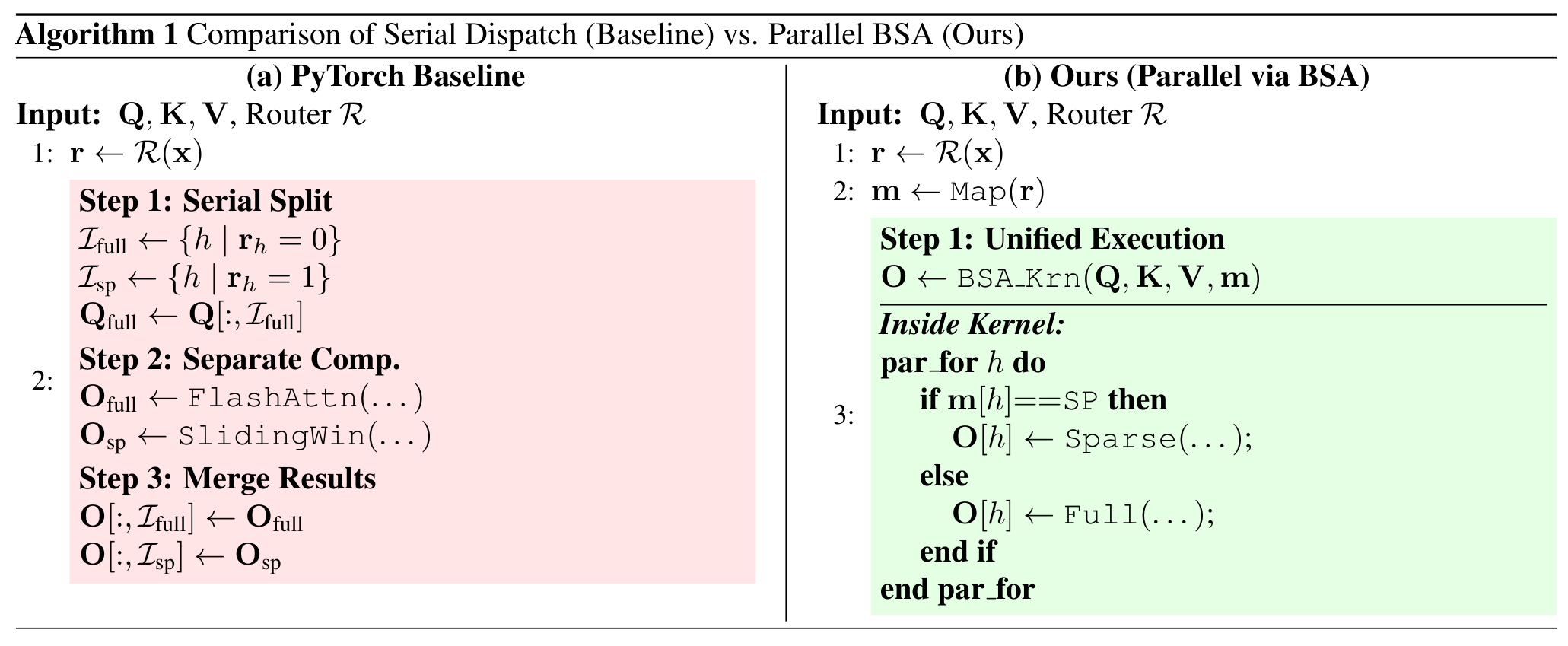
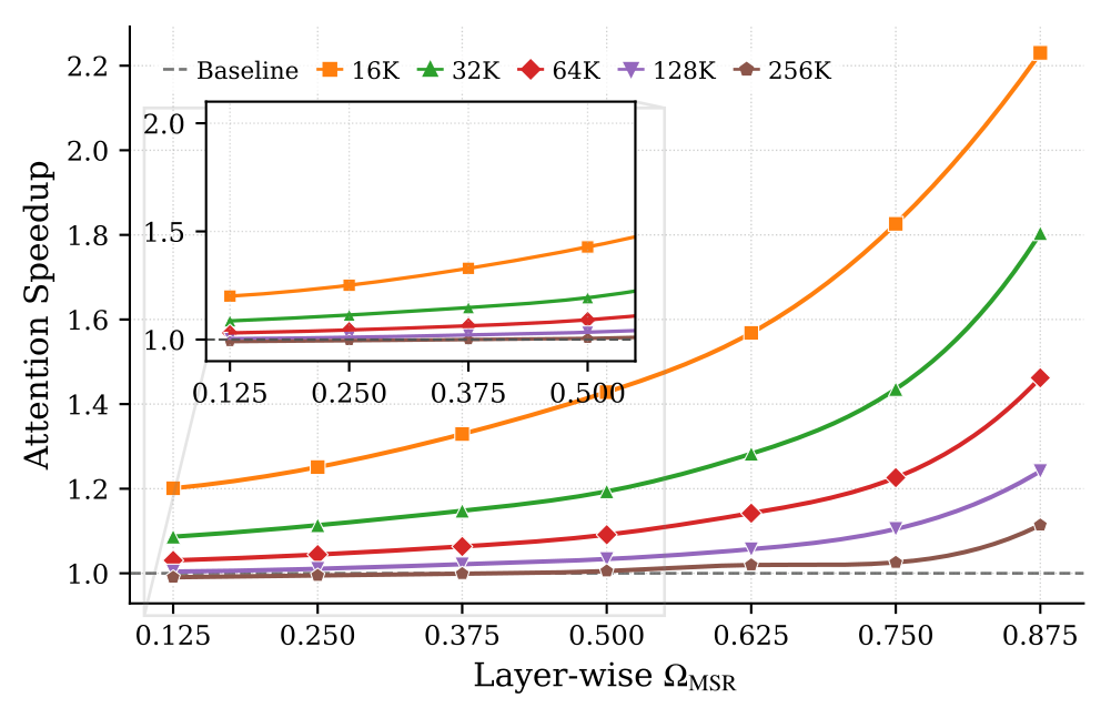
Figure 4: 融合 kernel 相对 Torch 顺序实现的注意力加速 — **Figure 4:**Comparison of our fused kernel with a Torch-based sequential implementation for layer-wise hybrid attention. 横轴为每条注意力层的模型稀疏比 $\Omega_{\text{MSR}}$(0.125–0.875),纵轴为加速比,四条线对应 16K/32K/64K/128K/256K 序列长度。两层信息:①同一稀疏比下,序列越长加速越明显(序列维并行是长上下文的主力,也正是碎片化伤害最大的地方);②同一长度下,稀疏比越高加速越大(被"省掉"的 SA 计算越多)。这张图是"kernel 融合不是锦上添花,而是混合头方案能否部署"的证据。报告 p.4

路由器本身的开销也要算清:它是每个 prefill 都要跑一遍的额外前向。

Figure 10: Router 延迟分析 — **Figure 10:**Router latency analysis. The router incurs negligible overhead (avg. 0.196 ms). Our design ensures length-invariant stability, maintaining constant speed from 512 to 1M tokens. 路由平均延迟仅 **0.196 ms**,且从 512 到 1M token 基本恒定——因为 Router 的输入是首尾各 100 token 的池化表征,与序列总长无关。这是"边界池化"设计的另一重收益:不仅提升任务识别信噪比,还让路由开销变成常数。报告 p.22

适用范围(论文的坦白):这套设计明确面向单卡部署的中小规模模型(单 GPU 或少量设备)。超大规模模型常用头级并行(不同头分到不同设备),那会与"逐层混合头"的结构冲突——论文在 Impact Statement 里主动划定了这个边界。

小结:部署这一章解决的问题是"动态路由不能被系统开销吃掉"。两个关键数字:融合 kernel 带来最高 2.2× 的注意力加速(Figure 4),Router 自身只花 0.196 ms 且与长度无关(Figure 10)。前者靠把路由决策下沉成 kernel 元数据,后者靠边界池化。

06 · Experiments

实验:三基准 × 三骨干

设置(整理自 §4.1 与附录 C):骨干为 Qwen3-4B、Qwen3-8B 与 Llama-3.1-8B-Instruct;训练数据由 5 个来源合成(ChatQA2-Long-SFT、MuSiQue、CoLT-132K、GovReport、XSum),共约 0.74B token,覆盖鲁棒型(代码补全、摘要、上下文学习)与敏感型(单文档 QA、多跳 QA)任务,序列长 8K–64K;目标稀疏比 $t_{\text{rob}}=1.0$、$t_{\text{sen}}=0.7$;8×A800 训练,单次 12 小时内;对比方法包括 DuoAttention、PruLong、InfLLM-V2(训练式)与 MoBA、NSA、XAttention(其他路线),评测统一走 LOOM-Eval 框架。稀疏头的实现有 SSA(流式稀疏)与 XA(XAttention)两种,记法"检索头模式-稀疏头模式",如 FA-SSA。

主结果 ①:LongBench-E(真实长上下文任务)

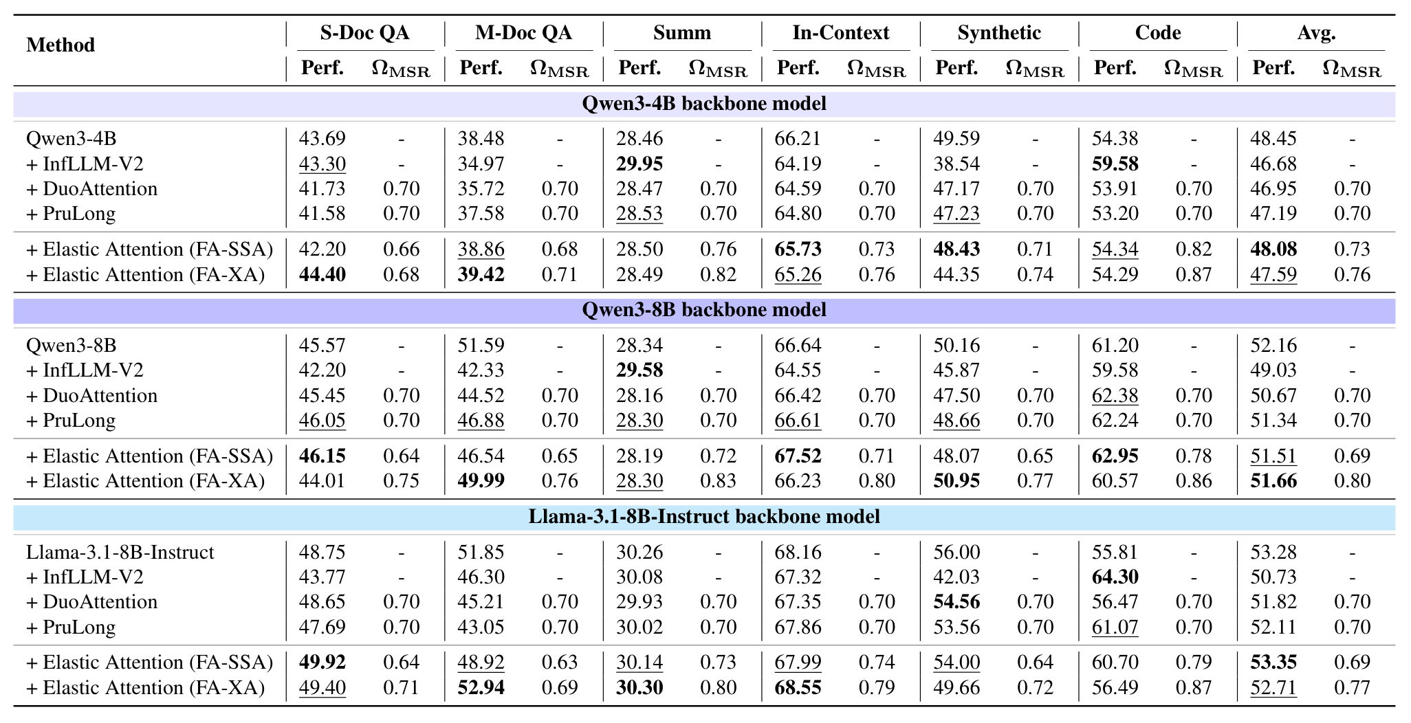
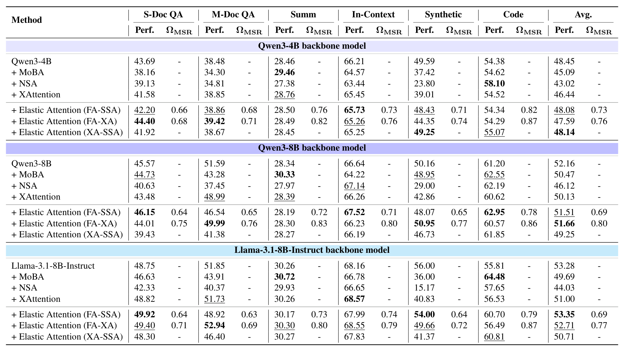
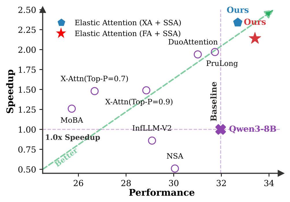
Table 1: LongBench-E 主结果(6 类任务 × 3 骨干) — **Table 1:**Performance on LongBench-E (Bai et al., 2024). We report average performance (Perf.) and $\Omega_{\text{MSR}}$ per task category. The 1st and the 2nd performance in each comparison group are highlighted with bold font and underlined, respectively. 三个骨干各成一组,每组内所有方法共享同一骨干与训练数据。Elastic Attention 在三组里都拿下平均分第一:Qwen3-4B 48.08(骨干全注意力 48.45、DuoAttention 46.95)、Qwen3-8B 51.51(骨干 52.16、PruLong 51.34)、Llama 53.35(超过骨干的 53.28)。更值得注意的是每个任务列的 $\Omega_{\text{MSR}}$:模型把稀疏比按任务拉开——代码类 0.78–0.82、摘要 0.72–0.73、单/多文档 QA 0.63–0.68。合成任务与上下文学习也没有被牺牲。论文也如实报告:在 Code/Summ 等鲁棒任务上个别基线略高,原因一半来自本文分配了更高的稀疏比。报告 p.5

主结果 ②:RULER 与 LongBench-V2(长度外推 + 长程推理)

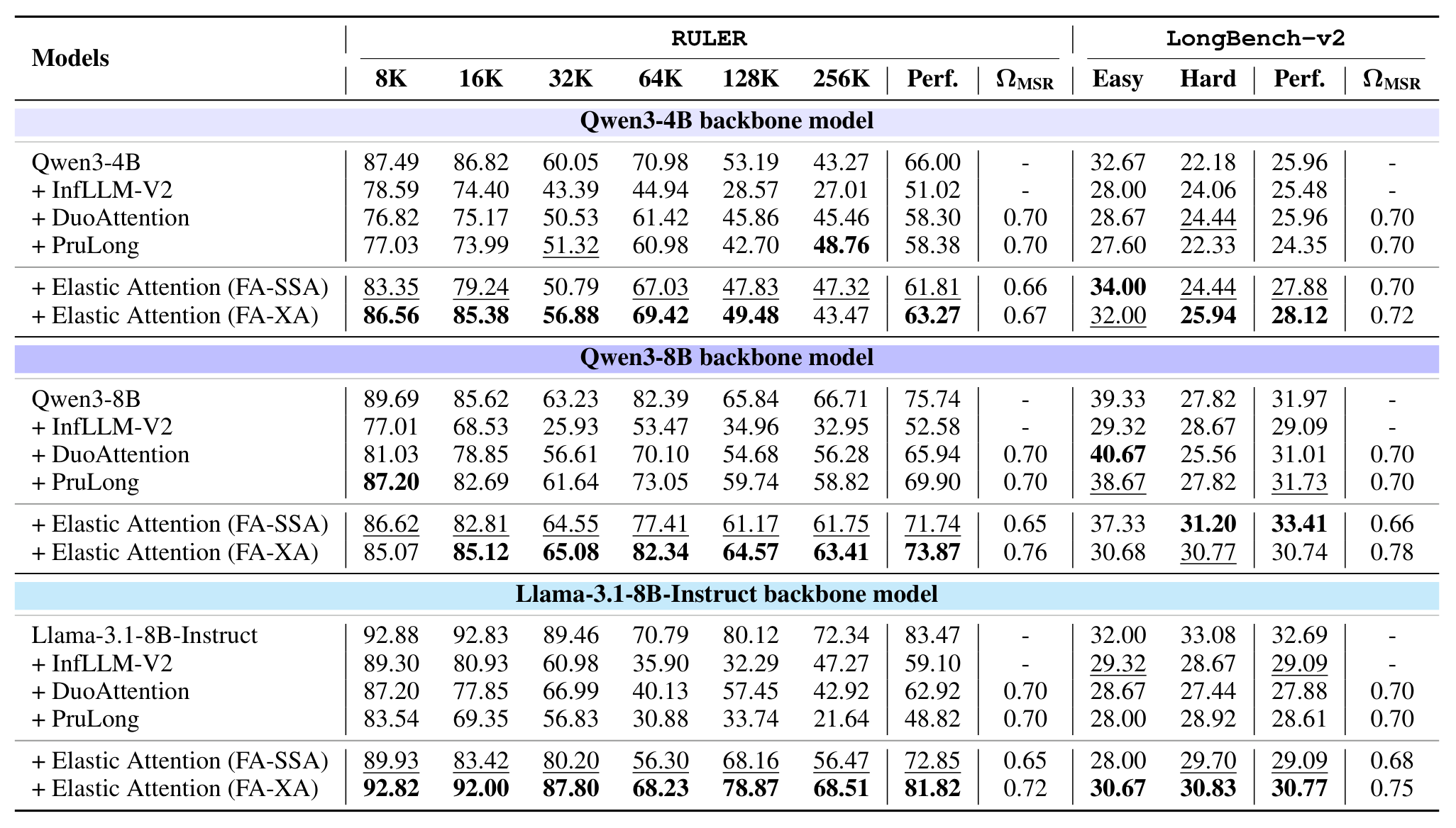
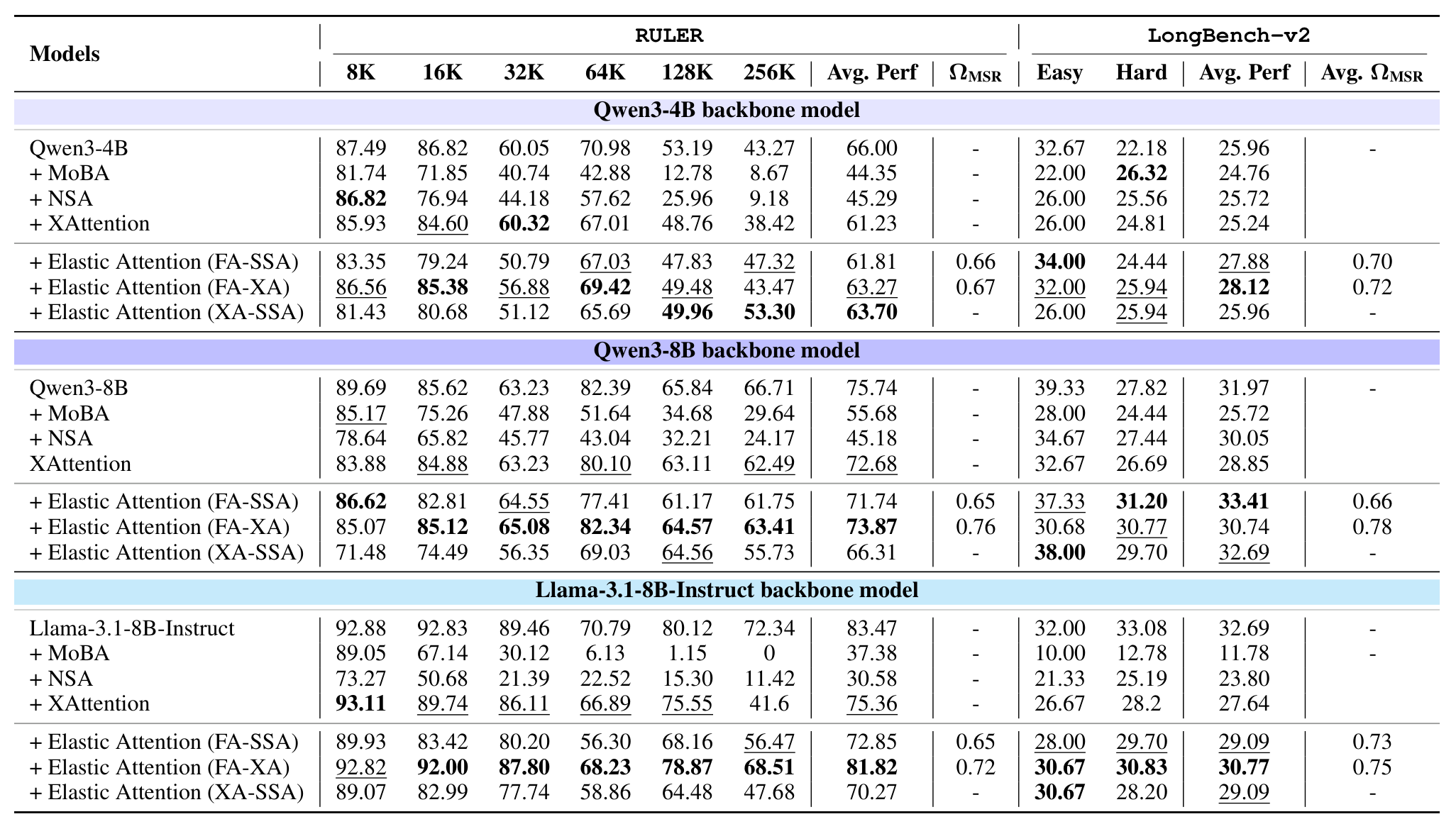
Table 2: RULER(8K–256K)与 LongBench-V2 结果 — **Table 2:**Model performance on RULER (Hsieh et al., 2024) and LongBench-v2 (Bai et al., 2025). We report the average Perf. and $\Omega_{\text{MSR}}$. 训练最长 64K,评测外推到 256K。左组 RULER:FA-XA 在 4B 上把平均分做到 63.27(vs 骨干 66.00),8B 上 73.87(vs 75.74),Llama 上 81.82(vs 83.47);同价位上 DuoAttention 只有 58.30/65.94/62.92,PruLong 58.38/69.90/48.82——静态比例方法在超长外推区间掉得更快。右组 LongBench-V2:Elastic Attention 在两个 4B/8B 骨干上都反超全注意力骨干(27.88 / 33.41 vs 25.96 / 31.97),Llama 上基本持平。论文特别指出:8B 级别、上下文超过 64K 后,FA-XA 之所以最优,是因为它的 $\Omega_{\text{ESR}}$ 更低——保留了更多有效信息(见 Figure 8c 的公平口径)。报告 p.6

主结果 ③:数学推理与领域长文档

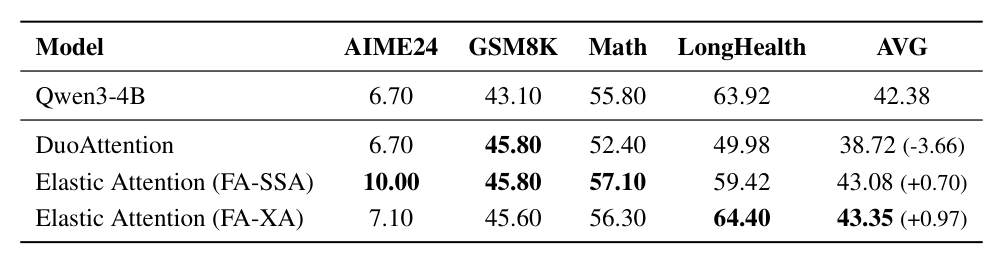
Table 3: AIME24 / GSM8K / Math / LongHealth 对比 — **Table 3:**Performance comparison across different benchmarks. The best results in each column are highlighted in bold. The values in parentheses indicate the performance gap relative to the Qwen3-4B baseline. Qwen3-4B 骨干上的四项考核:FA-SSA 在三个数学基准上全面最好(AIME24 6.70→10.00、GSM8K 43.10→45.80、Math 55.80→57.10),FA-XA 在医学长文档 LongHealth 上拿到 64.40。平均分:骨干 42.38,FA-SSA 43.08(+0.70),FA-XA 43.35(+0.97),而 DuoAttention 因 LongHealth 大跌而平均 38.72(-3.66)。**"稀疏=掉分"在这里被反例打破**:适度的稀疏化反而像一种正则,把成绩抬了起来。报告 p.6

效率与有效稀疏:一张图看三个指标

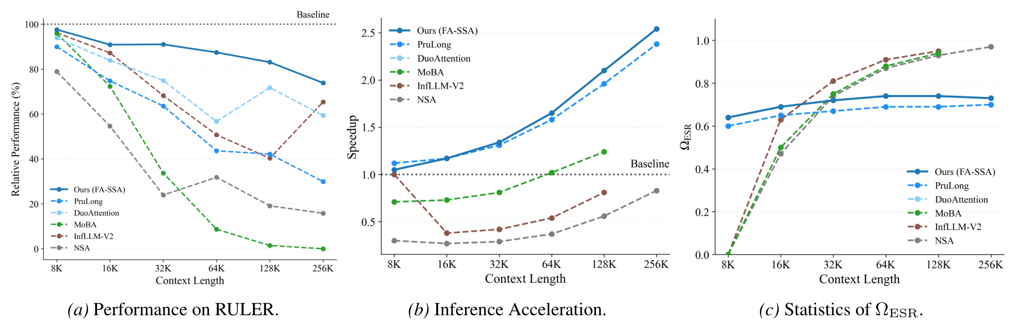
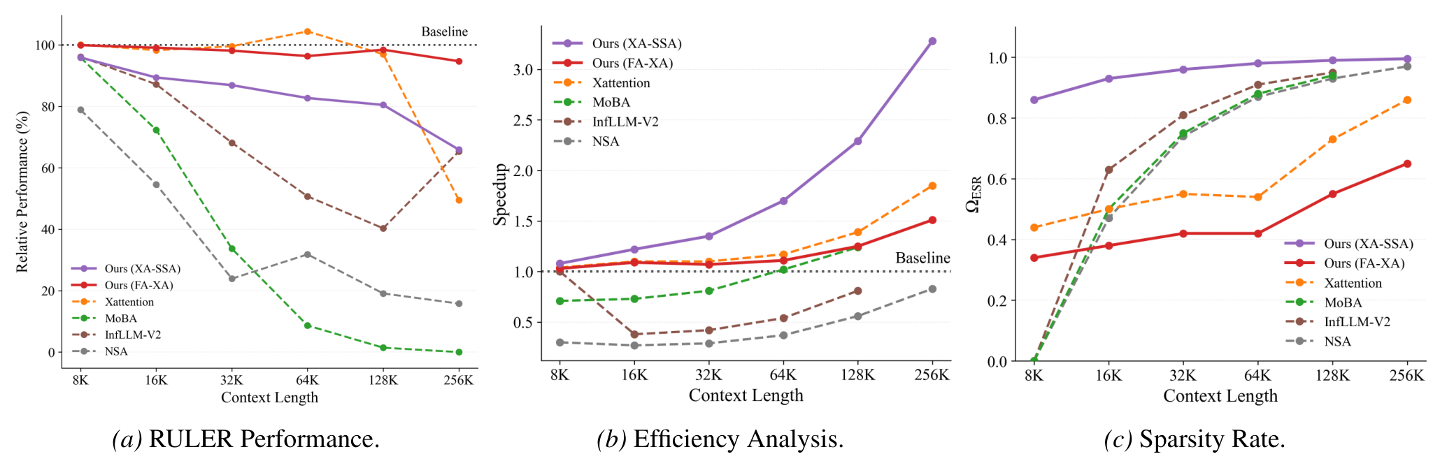
Figure 8: RULER 上的性能、加速与 Ω_ESR 统计 — **Figure 8:**Comparison of performance and inference speedup on the RULER benchmark across different methods. We adopt Llama-3.1-8B-Instruct as the backbone model and compare with training-based methods (FA-SSA), as well as other cutting-edge sparse attention methods. We report $\Omega_{\text{ESR}}$, as it provides a fair comparison of the effective proportion of attended tokens across different approaches. (a) 性能:各上下文长度分组,本文方法全面最好;(b) 加速:随上下文变长,本文的加速持续上扬——因为模型对更长的输入自动分配更高的稀疏比;(c) $\Omega_{\text{ESR}}$ 统计:训练式混合方法(如 DuoAttention)的有效稀疏比在各长度上基本恒定,而本文方法始终更低且随长度略有收缩——同样的"省算力"标称下,本文保留了更多实际参与的 token。论文还列举了两类竞争对手的系统性缺陷:NSA/InfLLM-V2 对 KV 头数有整除约束、与 Llama 头数不合;MoBA/InfLLM-V2 需预留预算做序列级特征,在 256K 处直接 OOM。报告 p.9

可扩展性:全稀疏区间与继续预训练

把检索头也换成 XAttention(XA-SSA 设置),整个模型进入全稀疏区间——这是对"弹性"上界的压力测试:

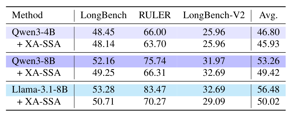
Table 5: XA-SSA(全稀疏)设置的结果 — **Table 5:**Results of implementing retrieval heads with XA. 三骨干三个基准的平均分对比:Qwen3-4B 上全稀疏只差 0.87 分(46.80→45.93),几乎无损;Qwen3-8B(53.26→49.42)与 Llama(56.48→50.02)出现可测退化——但换来的是整模型无 FA 头的加速结构。论文把这条曲线定义为"极端效率区间":精度与吞吐在此明确互换,选择权交给部署方。报告 p.8

另一条扩展线是打破"骨干冻结"约束:用 LoRA 与全参微调继续预训练,看路由能否与骨干协同进化。

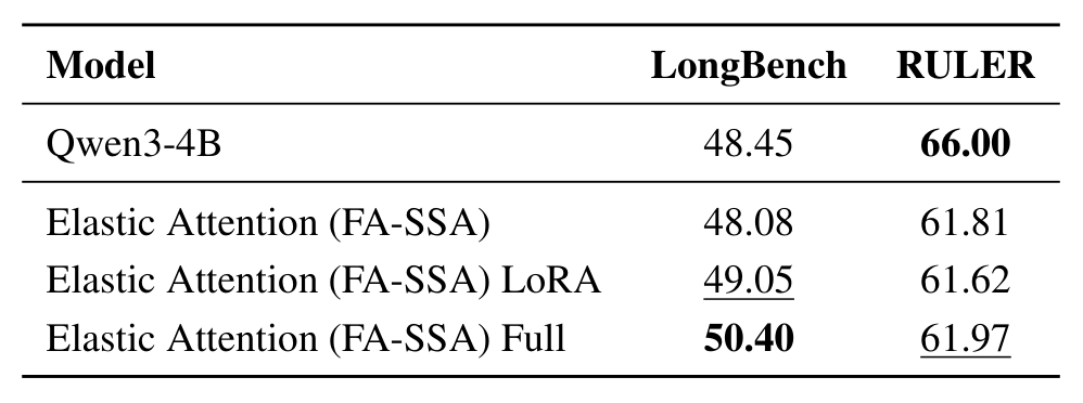
Table 6: 冻结 / LoRA / 全参微调三种模式对比 — **Table 6:**Performance comparison of different tuning methods on LongBench and RULER. The best results are bolded, and the second-best are underlined. Qwen3-4B 上:冻结骨干 48.08 → LoRA 49.05 → 全参微调 50.40(LongBench);RULER 上三者几乎持平(61.81 / 61.62 / 61.97)。释放更多参数能提升通用任务成绩,而合成检索性能(即长上下文能力)不降——说明 Elastic Attention 与继续预训练兼容,不会牺牲预训练模型已有的检索头。报告 p.8

小结:实验章的核心证据链是"三同一异":同骨干、同数据、同评测下,Elastic Attention ①在 LongBench-E 三组全部平均第一;②在 RULER 的超长外推区间优势最大;③在 LongBench-V2 上反超全注意力骨干;④数学与领域任务不降反升。而它的代价项只有训练 12 小时与 +0.27M/层。

07 · Analysis

消融与分析:路由学到了什么

目标稀疏比 $t$ 怎么选

训练时给敏感任务的目标稀疏比 $t_{\text{sen}}$ 是一个人为设定的先验。论文把 $t_{\text{sen}}$ 从 0.7 一路降到 0.4,观察模型的实际分配:

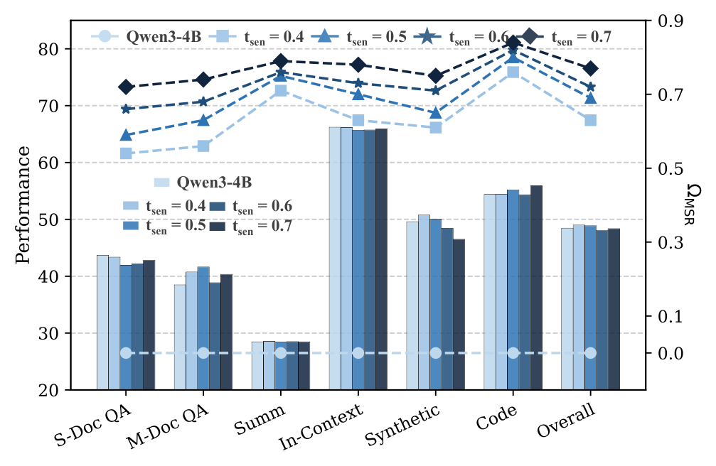
Figure 7: 不同目标稀疏比 t 设置下的性能与实测 Ω_MSR — **Figure 7:**Comparison of performance and test-time $\Omega_{\text{MSR}}$ among different training sparsity target $t$ settings. The bar chart denotes the performance and the line chart denotes $\Omega_{\text{MSR}}$ in each task. 柱=各任务性能,线=实测 $\Omega_{\text{MSR}}$。$t_{\text{sen}}$ 越小,任务间的稀疏比分化越明显(约束越松,模型越敢按任务拉开档位);$t_{\text{sen}}$ 低到 0.4 时整体性能甚至能超过全注意力骨干。但论文最终仍选 $t_{\text{sen}}=0.7$——从推理效率角度,"留出稀疏空间"比"多挤一点分数"更符合方法初衷。这条曲线也说明:**目标值 $t$ 不是硬指标,而是给模型的建议区间**,实测 $\Omega_{\text{MSR}}$ 并不严格等于 $t$。报告 p.7

Router 的结构消融:要多大、为什么要两段 MLP

Table 4: Router MLP 中间隐维的消融 — **Table 4:**Comparison among different MLP hidden dimensions. 中间隐维从 $2\times d'$ 试到 $8\times d'$($4\times d'$ 为默认):各设置平均分差距很小(45.22 / 45.92 / 45.45 / 46.40),$8\times d'$ 略高但参数更多——论文选择 $4\times d'$ 作为性能与参数开销的折中。这说明路由能力主要来自"任务表征"这一层抽象,而不是 MLP 的容量。报告 p.7

Task MLP 的作用可以直接可视化:看同一批输入在 MLP 前后的任务表征相似度。

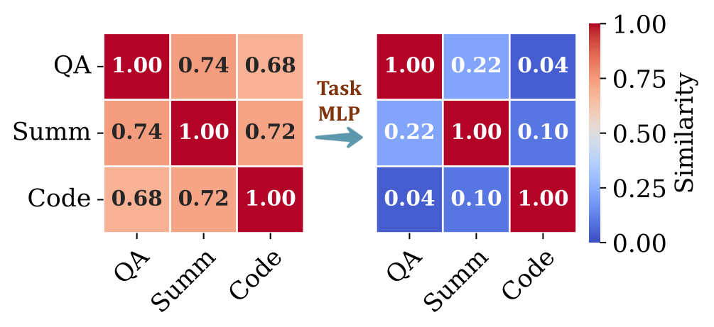
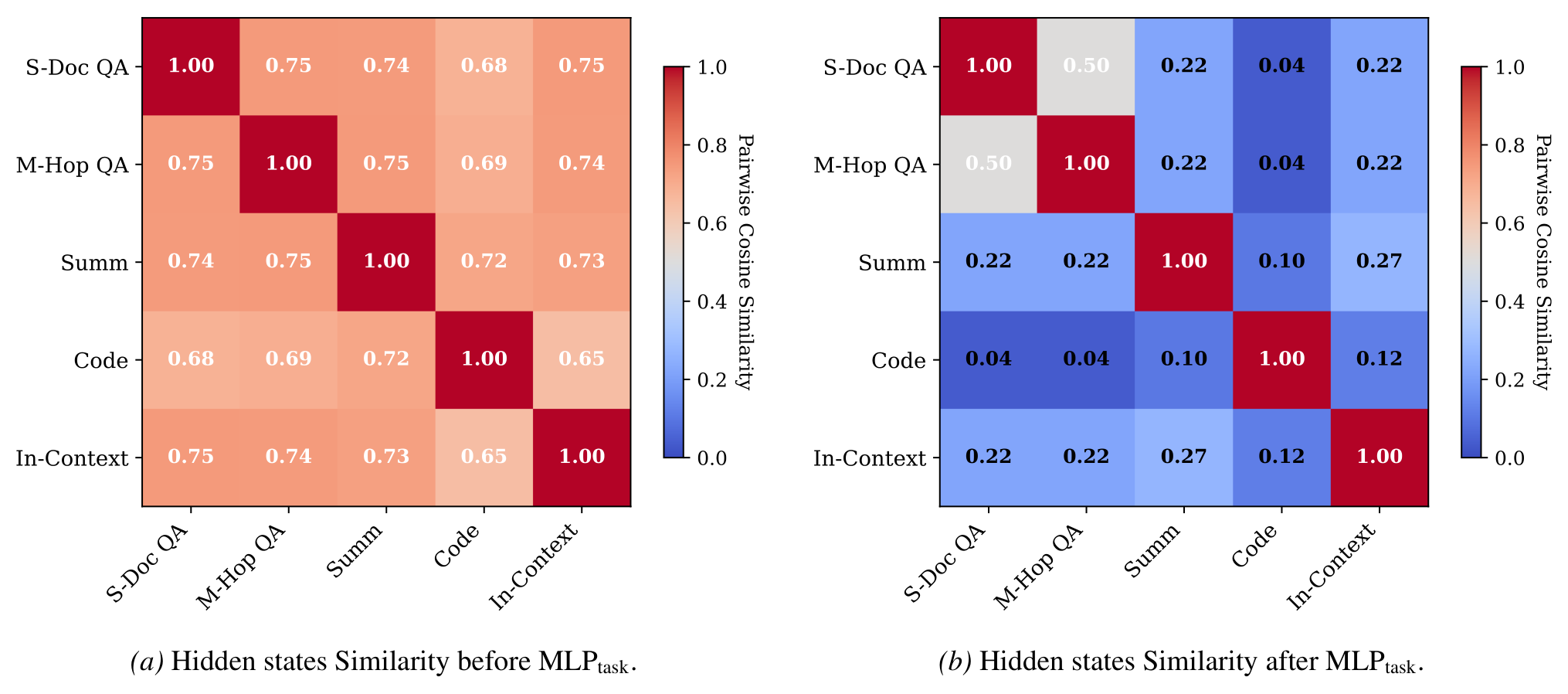
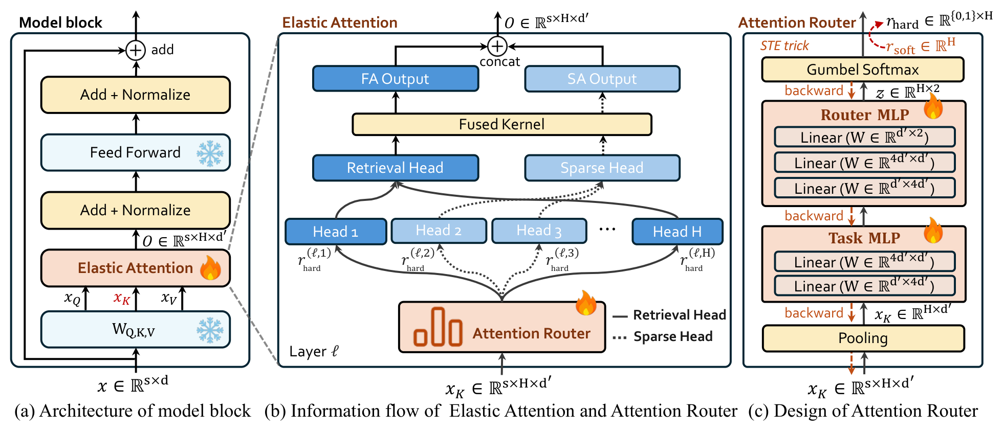
Figure 5: Task MLP 前后的任务表征相似度 — **Figure 5:**Visualization of task representation similarity. (Left) before Task MLP, the pooled hidden states exhibit high pairwise cosine similarity across different tasks; (Right) after passing through the Task MLP, the inter-task similarity significantly decreases. 左:池化隐状态在不同任务之间高度相似(表征还没"分家");右:过完 Task MLP 后任务间相似度显著下降。也就是说,**Task MLP 干的是"把任务特征从通用隐状态里解耦出来"**,为后面的 Router MLP 提供可判别的输入。附录 G.1 用更严格的 pairwise conditional rescaling 度量给出同一结论: 报告 p.7

Figure 9: 路由表征的成对余弦相似度(正交子空间证据) — **Figure 9:**Pairwise cosine similarity of routing representations $z_{\text{task}}$. The prevalence of near-zero scores ($M_{uv}\approx 0$) indicates that the router maps distinct tasks to orthogonal subspaces on the local manifold. This confirms that the model implicitly disentangles task semantics into independent directions without supervision. (a) MLP 前、(b) MLP 后:大量任务对的相似度趋近于 0,意味着 Task MLP 把不同任务映射到了局部流形上的**近似正交子空间**。注意这一切没有任务标签监督——纯粹是"稀疏-性能"目标逼出来的副产品。这是全文最有信息量的一张"机制图"。报告 p.22

路由模式长什么样

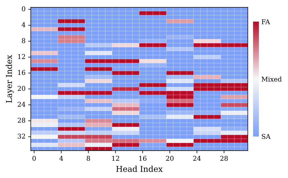
Figure 6: Qwen3-4B 每个头的路由激活频率 — **Figure 6:**Overview of routing activation frequency of each head in Qwen3-4B. Red indicates heads that are consistently routed to FA (i.e., retrieval heads) across all 6 tasks in LongBench-E, while blue denotes heads that are consistently routed to SA. 横轴=头序号,纵轴=层序号,颜色=6 个任务上被路由到 FA 的频率(红=总是 FA,蓝=总是 SA,浅色=随任务切换)。可以看到:①一小撮头(集中在**中高层**)稳定走 FA——与 Retrieval Head 论文发现的"检索头"位置一致;②有部分头随任务切换(浅色),这正是"弹性"发生的地方;③其余头稳定走 SA。路由不是随机噪声,而是复现了已知的模型结构。报告 p.7

换一个模型家族,模式却不一样——这是论文里少见的跨模型机制发现:

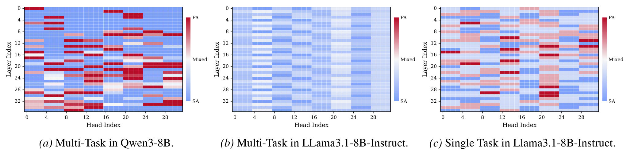
Figure 11: 跨模型的路由鲁棒性分析 — **Figure 11:**Extended Head Robustness Analysis. Similar to Figure 6, these heatmaps visualize the frequency of full-attention activation for each head. (a) and (b) show the multi-task global robustness for Qwen3-8B and Llama3.1-8B-Instruct, respectively. (c) presents the robustness analysis for Llama3.1-8B-Instruct in a single-task setting. (a) Qwen3-8B:存在一批"跨任务恒定激活/恒定稀疏"的头——**任务无关的注意力拓扑**;(b) Llama-3.1-8B 的多任务聚合视图里找不到恒定激活的头;(c) 但拆到单任务看,强激活头是存在的,只是随输入动态迁移。结论:Qwen3 依赖固定的检索头,而 Llama-3.1 会按任务重新分配注意力资源——**同一套路由机制,在两个模型家族里学出了不同的策略**。报告 p.22

训练动态:路由是"学"出来的

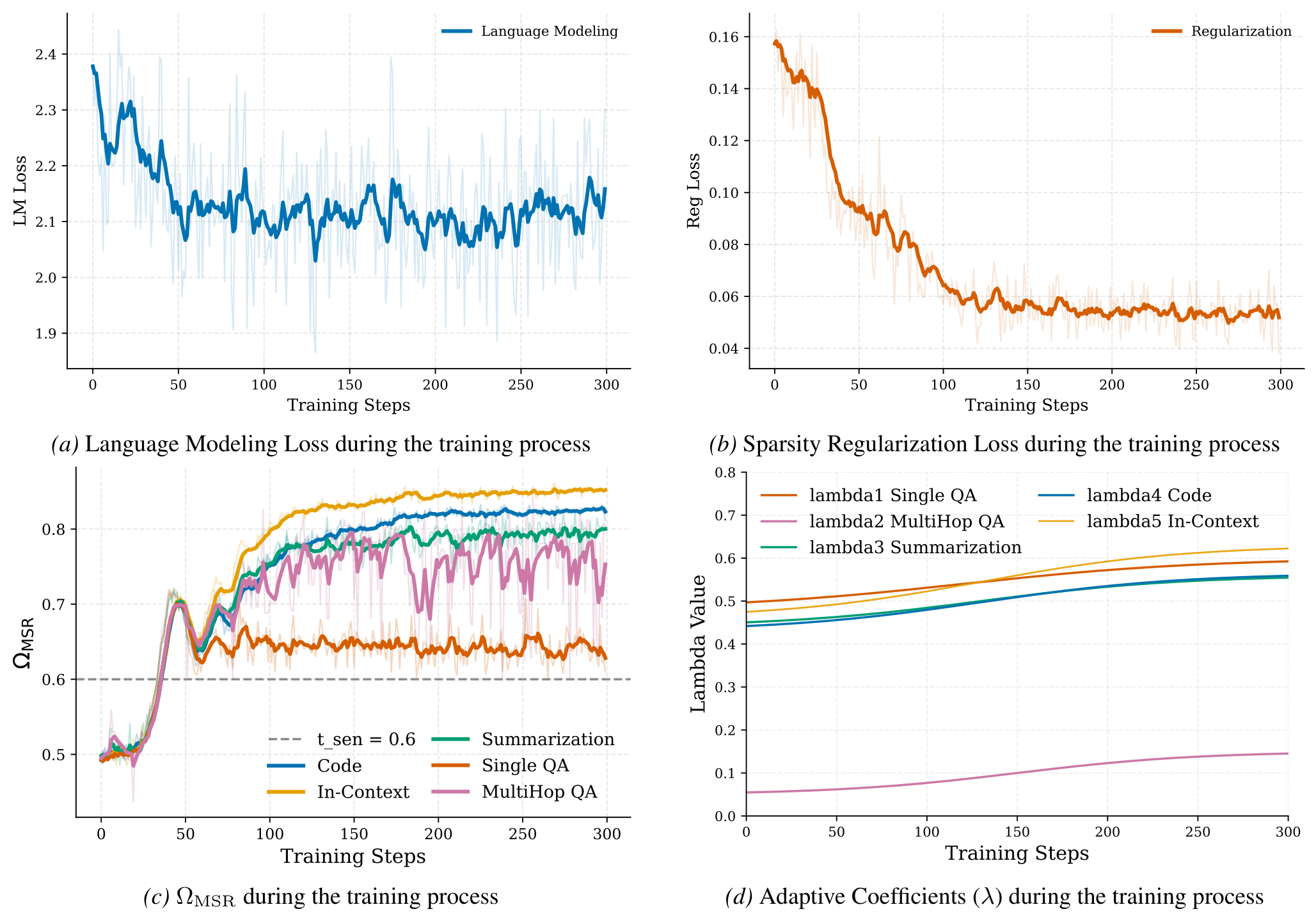
Figure 13: 训练四视角(LM 损失 / 正则损失 / Ω_MSR / λ) — **Figure 13:**Decomposition of Training Objectives for Elastic Attention. We visualize the training dynamics of the Attention Router, separating the total loss into (a) the primary language modeling objective and (b) the sparsity regularization term. Subfigures (c) and (d) illustrate the task-level differentiation in sparsity allocation ($\Omega_{\text{MSR}}$) and adaptive coefficients ($\lambda$), demonstrating how the model automatically distinguishes between sparsity-robust and sparsity-sensitive tasks. (a) 语言建模损失快速下降并稳定在 ~2.1——注入稀疏没有妨碍骨干收敛;(b) 稀疏正则损失在前 100 步从 ~0.16 降到 ~0.06——Gumbel 松弛把路由器"推"向目标稀疏比;(c) 各任务的 $\Omega_{\text{MSR}}$ 从中性初始化出发自动分化:代码/上下文学习收敛到 ~0.80–0.85(接近甚至超过 $t_{\text{sen}}$ 方向),Q&A 则停在更接近目标线的位置;(d) 拉格朗日乘子的演化:$\lambda_5$(上下文学习)涨得最猛——模型把"满足这个任务的密度要求"排在了最优先。300 步训练全程稳定。报告 p.24

路由输入要多长才够

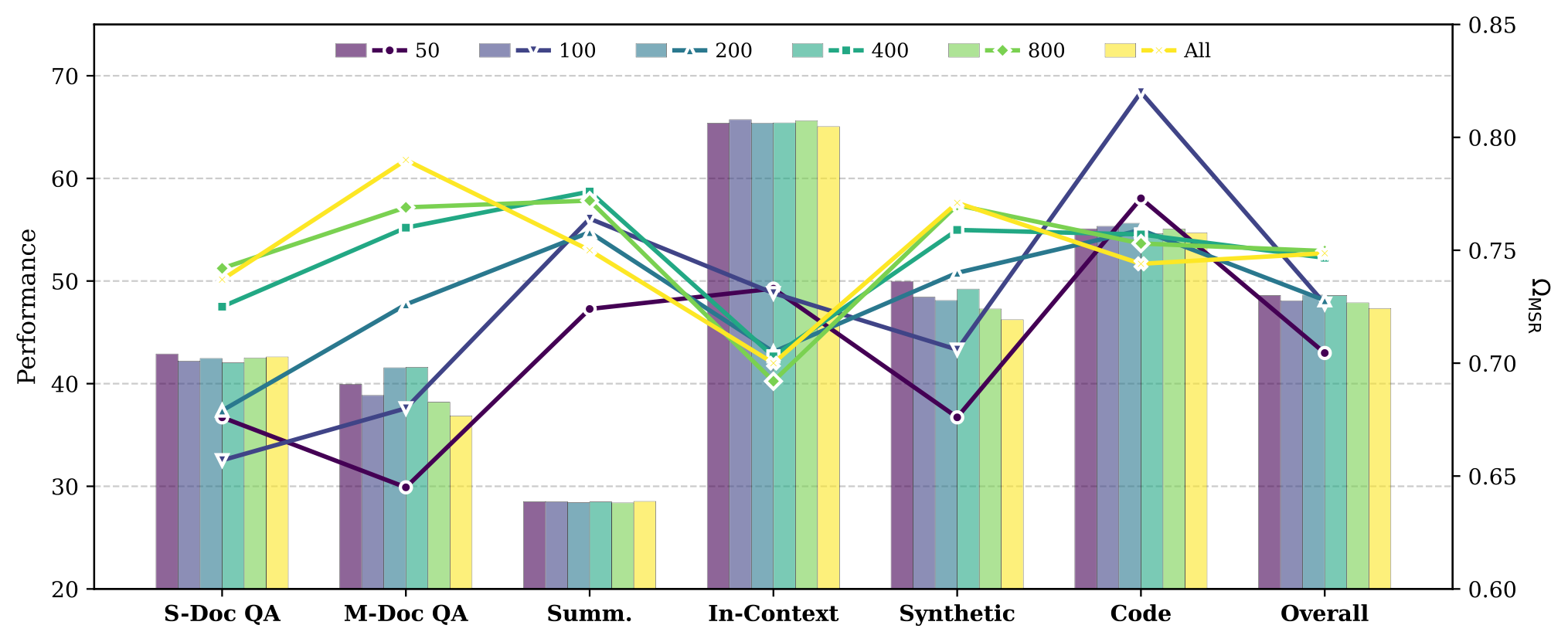
Figure 14: 路由输入截断长度的影响 — **Figure 14:**Impact of router input truncation length on downstream performance and $\Omega_{\text{MSR}}$. We compare varying truncation budgets ($L\in\{50,\dots,800,\text{All}\}$) applied to the concatenation of the sequence's prefix and suffix. Results indicate that increasing the input length beyond 100 tokens yields negligible performance gains and may degrade router selectivity due to a lower signal-to-noise ratio. 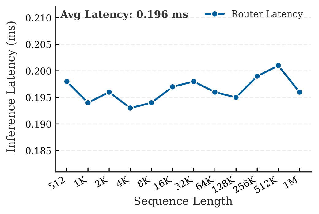把路由输入的首尾预算从 50 加到 800、再到全序列:性能在 **100–200 token 处就饱和**,继续加长不再有收益,某些任务(如多文档 QA)反而变差——因为文档正文的语义方差把"系统提示 + 用户问题"的信号稀释了。这是"边界池化 100+100"配置的直接实验依据,也解释了 Figure 10 里路由延迟为什么与序列长度无关。报告 p.25

长度外推与稀疏动态

小结:分析章的四个发现——①Task MLP 让任务表征正交化(无监督地);②路由模式复现了检索头的已知结构,且在不同模型家族中策略不同;③训练 300 步内自动完成任务分化,拉格朗日乘子按任务"抢预算";④路由输入只需首尾 100 token。这些证据共同支撑一个判断:模型内部本来就存在"任务敏感性"的可分结构,路由器只是把它读了出来。

08 · Appendix

附录:复现细节、更多结果与案例

训练超参与评测配置

Table 8: 训练超参与基线专有配置 — **Table 8:**Hyperparameters: General configuration (Left) and Baseline-specific settings (Right). 左表(通用配置):序列长 65,536、bfloat16、全局批 48、300 步、Router/正则学习率 $5\times10^{-4}$/$1\times10^{-3}$、warmup 0.2、AdamW $(\beta_1,\beta_2)=(0.9,0.95)$、weight decay 0.1、余弦退火;稀疏配置:sink/local 128/2048、block/chunk 64/16384、stride/threshold 16/0.9。右表(基线专有):MoBA/NSA/InfLLM-V2 的块大小(1024/64/64)、Top-k(8/128/64)、窗口(–/512/2048)等——论文强调所有基线都在同一环境与数据上重训,并严格沿用各自原论文的超参。报告 p.16

Table 11: RULER 评测配置 — **Table 11:**Detailed configuration for the RULER benchmark evaluation. We evaluate across exponentially increasing context windows up to 256k tokens. RULER 的评测口径:8K–256K 六个长度;每个"任务×长度"对 50 个样本;任务含 NIAH 检索系列(single/multikey/multiquery/multivalue 各 1–3 档)与 QA/抽取系列(qa1/qa2、fwe)。这些细节决定了横向对比的可比性,报告得比较完整。报告 p.20

LongBench-E 逐任务明细

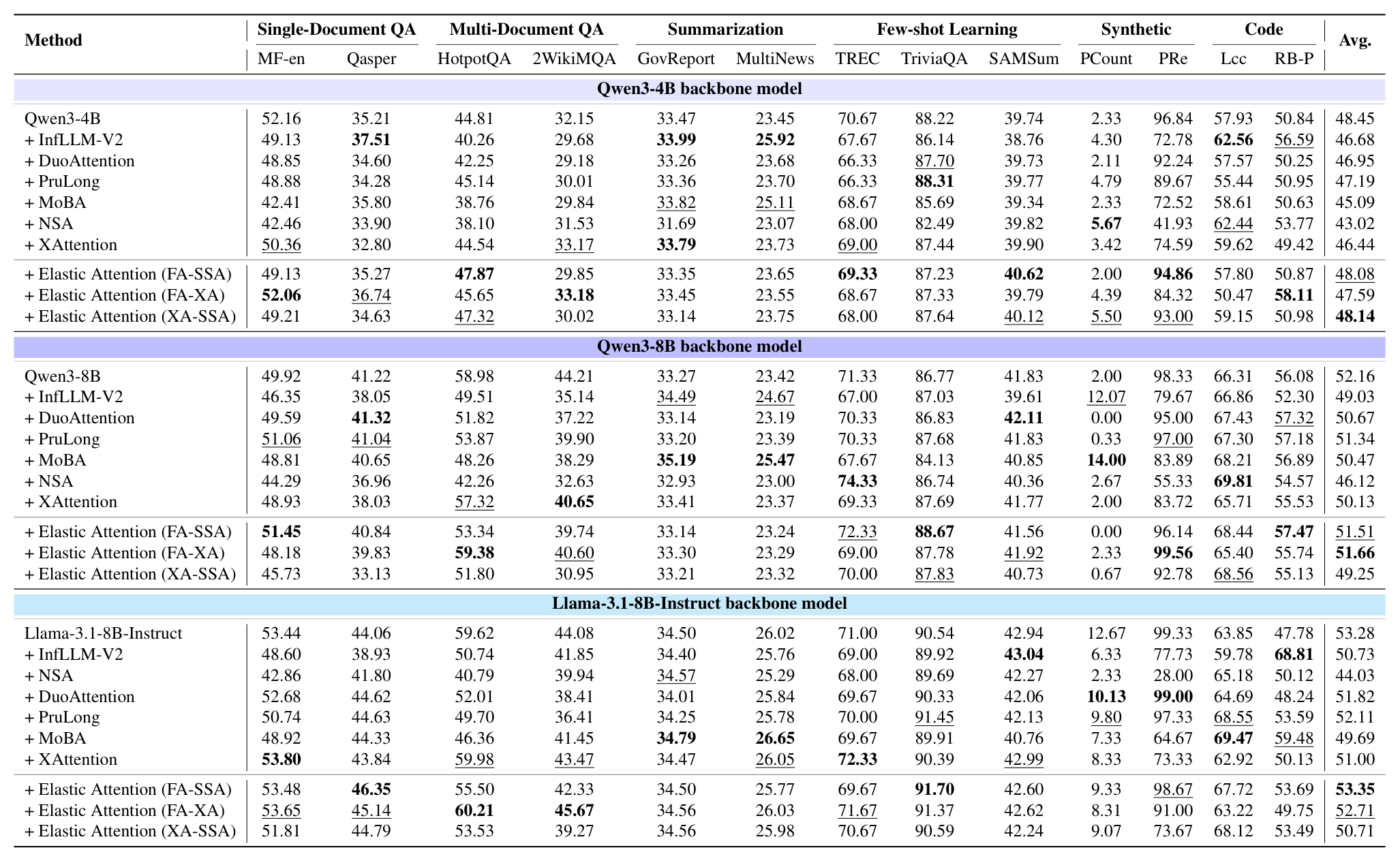
Table 9: LongBench-E 14 项子任务完整结果 — **Table 9:**LongBench-E results comparison. The 1st and the 2nd performance in each comparison group are highlighted with bold font and underlined, respectively. 全部 13 个子任务(MF-en、Qasper、HotpotQA、2WikiMQA、GovReport、MultiNews、TREC、TriviaQA、SAMSum、PCount、PRe、Lcc、RB-P)的分数,三个骨干分组对比 InfLLM-V2 / DuoAttention / PruLong / MoBA / NSA / XAttention 与 Elastic 的两种设置。读法建议:先看自己关心的任务列,再回头看该组平均。报告 p.18

Table 10: LongBench-E 分类别性能与 Ω_MSR(含 MoBA/NSA/XA-SSA) — **Table 10:**Performance on LongBench-E. We report average performance (Perf.) and $\Omega_{\text{MSR}}$ per task category. The 1st and the 2nd performance in each comparison group are highlighted with bold font and underlined, respectively. 与 Table 1 同构的补充版,额外纳入 MoBA、NSA 与 XA-SSA(全稀疏),并按类目给出 $\Omega_{\text{MSR}}$。可以直观看到 Elastic 的稀疏比在**类目之间**的差异(如 Qwen3-4B:QA 0.66–0.68、代码 0.82、合成 0.71),而所有基线方法要么恒为 0.70、要么不定义 $\Omega_{\text{MSR}}$。报告 p.19

RULER / LongBench-V2 补充结果

Table 12: RULER 与 LongBench-V2 补充对比(含 MoBA/NSA/XAttention) — **Table 12:**Additional results on RULER and LongBench-v2. 把 MoBA、NSA、XAttention 与 Elastic 三种配置放在同一张逐长度表里。两个极端值得注意:Llama 骨干上 MoBA 从 32K 起雪崩(30.12 → 6.13 → 1.15 → 0),NSA 在 256K 只剩 11.42;而 FA-XA/XA-SSA 在 256K 仍分别有 68.51 / 47.68。这张表是"动态稀疏 vs 静态稀疏在外推区间差距"的最细颗粒度证据。报告 p.20

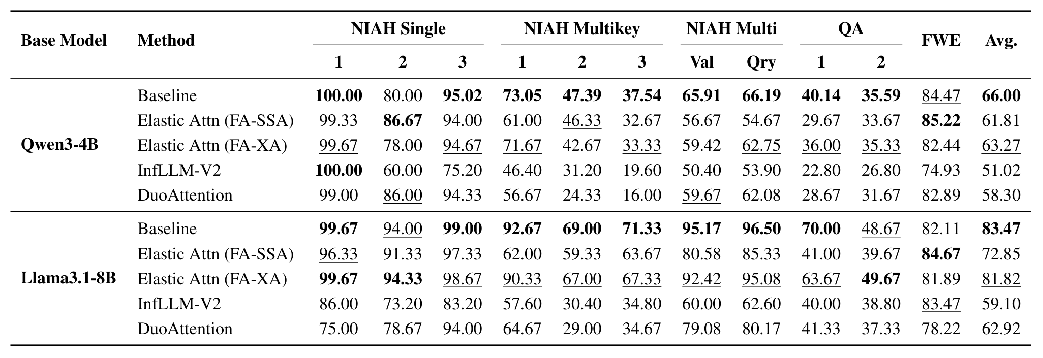
Table 13: RULER 子任务明细 — **Table 13:**Performance comparison of different attention methods on RULER subtasks. Tasks are grouped logically to highlight performance variations. RULER 子任务拆解(NIAH single/multikey/multi 的 Val/Qry、QA1/QA2、FWE)。一个有意思的模式:在 Llama 骨干上,Elastic(FA-XA)在 FWE(QA 类)上反而高于 Baseline(81.89 vs 82.11 基本持平,而 DuoAttention 只有 78.22)——稀疏化没有牺牲需要精细检索的子任务,掉分主要发生在最难的 NIAH multikey 多档。报告 p.21

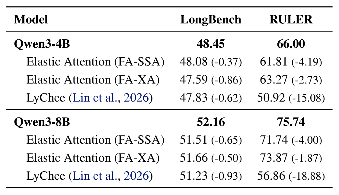
Table 14: 与 LyChee 的对比 — **Table 14:**Performance comparison on LongBench and RULER. The performance drop relative to the respective base model is shown in parentheses. 与同期混合头工作 LyChee(Lin et al., 2026)的正面对比:LongBench 上两者互有胜负(4B: -0.37 vs -0.62;8B: -0.65 vs -0.93),但 RULER 上差距拉开——Elastic 掉 4.19/4.00,LyChee 掉 **15.08/18.88**。长上下文外推是这类方法的分水岭。报告 p.21

定性案例:三场"细节决定成败"的对比

附录 H 给了三个真实案例,展示稀疏化误差会以什么形式出现——共同的失效模式是丢掉了关键细节,然后用通顺的话把它补圆:

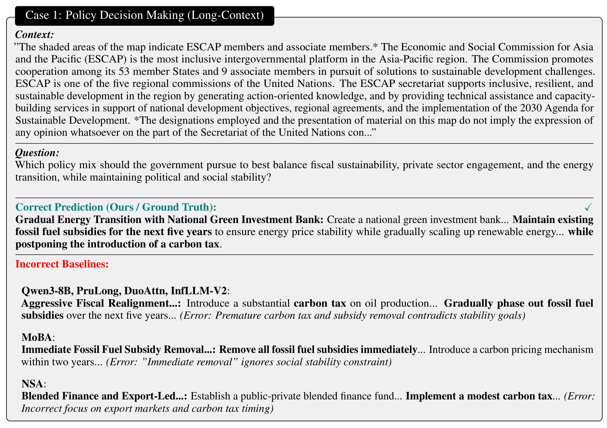
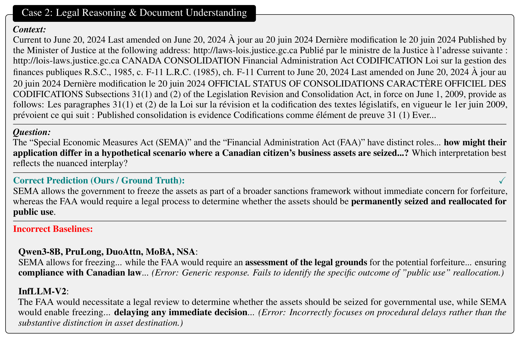
Figure 15: 政策推理案例的定性对比 — **Figure 15:**Qualitative comparison on a complex policy reasoning task. Our model correctly identifies the 'Gradual' approach required for stability, whereas baselines hallucinate 'Aggressive' or 'Immediate' measures that contradict the stability constraint. 案例 1(政策推理):问题要求在"财政可持续、社会稳走、能源转型"间找平衡。正确答案是"渐进式绿色投资 + 保留化石能源补贴五年 + 推迟碳税";Qwen3-8B / PruLong / DuoAttn / InfLLM-V2 给出"激进碳税 + 五年内退出补贴",MoBA 干脆"立即取消全部补贴"——都违反了"社会稳定"这一约束。Elastic Attention 抓住了"渐进"这个关键词。报告 p.26

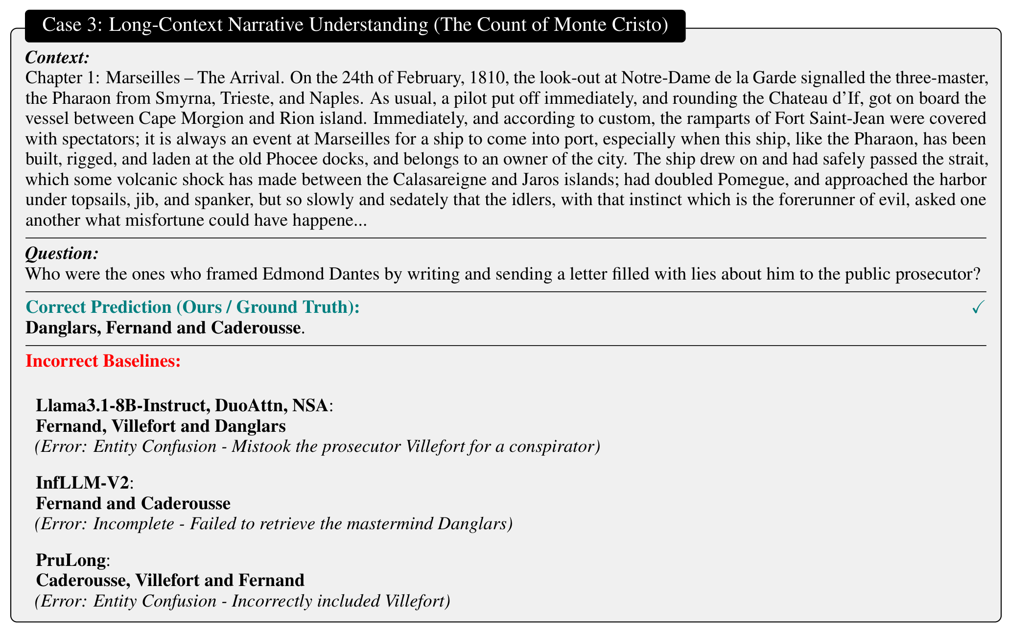
Figure 16: 双语法律文档案例 — **Figure 16:**Comparison on a bilingual legal document. Our model accurately extracts the specific legal provision regarding asset reallocation for public use (FAA), whereas baselines provide generic descriptions of “legal assessments” or “compliance” without specific details. 案例 2(双语法律):问 SEMA 与 FAA 在"资产被扣押"场景下的适用差异。正确回答需要点出 FAA 的"为公共用途重新分配";基线们给出的是"需要法律评估""确保合规"这类正确但无信息的泛泛之谈——典型的"稀疏丢失细节后靠语言先验补全"。报告 p.27

Figure 17: 叙事实体追踪案例 — **Figure 17:**Qualitative comparison on narrative entity tracking. The task requires identifying the specific characters who conspired to frame the protagonist. Our model accurately retrieves the correct trio, whereas baselines consistently hallucinate “Villefort” (the public prosecutor) into the group, failing to distinguish between the plotters and the judicial figure involved later. 案例 3(长篇小说实体追踪,约 5 万 token 的《基督山伯爵》):问"谁写了诬告信陷害主角"。正确答案是 Danglars、Fernand、Caderousse 三人;多个基线把后文才出场的检察官 Villefort 混进共谋者名单,InfLLM-V2 还漏掉了主谋 Danglars。实体关系细节正是稀疏化最容易伤到的部分——这也是 Elastic Attention 在敏感任务上把稀疏比压到 0.63–0.68 的原因。报告 p.28

编者注(论文笔误):附录 H 正文写"In Table 15, 16, and 17, we present representative model outputs",但这三个编号对应的实际是 Figure 15/16/17(定性案例),论文里不存在 Table 15–17。不影响结论,记录在此以免读者对着表格编号找半天。

Glossary

术语速查

阅读中遇到缩写,可随时回到这里;正文里带虚线下划线的缩写悬停即可见释义。

阅读术语表(正文中带虚线下划线的缩写悬停可见)
缩写	全称	一句话解释
FA	Full Attention	全注意力:每个 token 关注全部历史 token,精度的上限、成本的上限
SA	Sparse Attention	稀疏注意力:只保留一小部分 K/V 计算,省算力但可能丢细节
Ω_MSR	Model Sparsity Ratio	模型稀疏比:稀疏头占全部 KV 头的比例(定义 2.1)
Ω_ESR	Effective Sparsity Ratio	有效稀疏比:把每个头的剪枝率 ρ 也计进去的稀疏度(定义 2.2)
SSA	Streaming Sparse Attention	流式稀疏注意力:attention sink + 滑窗的静态稀疏模式(Xiao et al., 2024b)
XA	XAttention	训练无关的块稀疏注意力,用反对角线打分挑关键块(Xu et al., 2025)
BSA	Block-Sparse-Attention	块稀疏注意力内核,本文用它实现"混合头单次 launch"(Guo et al., 2024)
STE	Straight-Through Estimator	直通估计器:前向用硬决策、反向把梯度传给软分布
Gumbel-Softmax	—	用 Gumbel 噪声 + 温度把离散采样变成可导采样
DuoAttention	—	静态混合头基线:检索头走 FA、流式头走 SSA(Xiao et al., 2025)
PruLong	—	训练式 KV 剪枝基线(Bhaskar et al., 2025)
InfLLM-V2	—	可切换稠密/稀疏的注意力基线,短上下文用 FA(Zhao et al., 2025)
MoBA / NSA	Mixture of Block Attention / Native Sparse Attention	两个代表性稀疏注意力架构(块路由 / 原生可训练稀疏)
NIAH	Needle-in-a-Haystack	大海捞针:长上下文检索能力的经典探针,也是 RULER 的主任务族
RULER	—	可配置长度的合成长上下文评测,含检索与 QA/抽取(Hsieh et al., 2024)
LongBench-E / LongBench-V2	—	真实长上下文评测v1(14 任务)与其升级版 v2(8K–2M 词的长程推理)
FWE	Fuzzy Word Extraction	RULER 的模糊词抽取子任务,考察细粒度定位
LOOM-Eval	—	本文使用的长上下文评测框架(Tang et al., 2025)
LyChee	—	同期混合头稀疏解码工作(Lin et al., 2026),Table 14 的对比对象

10 · Commentary

点评与展望

论文自己的结论与局限

作者总结:把下游任务归为"稀疏鲁棒 / 稀疏敏感"两类,用一个轻量 Attention Router 做逐头 FA/SA 路由,就能在不修改预训练骨干、12 小时训练的前提下让模型按输入自动分配稀疏度;三个基准、三个骨干上的实验支持这一路线。作者主动交代的边界:①方法面向单卡/少卡部署的中小模型(大规模头级并行与逐层混合头冲突);②长上下文评测中,敏感任务的稀疏收益与精度之间仍需按场景取舍;③路由的"每请求一次"决策粒度也隐含在 prefill-stage 的设定里。

技术来源与继承(据论文引用整理)

论文对组件来源标注得比较完整,下表把散落正文与附录的引用汇总到一处,便于按"继承 → 改造"的视角重读:

技术来源一览(据论文行内引用整理,非论文原表)
组件	论文标注的上游	本工作的改造 / 集成
检索头概念与识别	Retrieval Head(Wu et al., 2024)	用作稀疏扫描实验的头排序依据(NIAH 探针打分 + 渐进替换)
混合头机制	DuoAttention(Xiao et al., 2024a; 2025)、PruLong(Bhaskar et al., 2025)	把静态比例改为输入自适应的逐头路由
稀疏头计算	Streaming Sparse Attention(Xiao et al., 2024b)、XAttention(Xu et al., 2025)	作为 SA 侧的两种可插拔实现(FA-SSA / FA-XA / XA-SSA)
稀疏 kernel	Block-Sparse-Attention(Guo et al., 2024)	把路由决策下沉为内核元数据,混合头单次 kernel launch
路由机制	MoE gating(Shazeer et al., 2017)	"选专家"改为"选注意力模式",粒度落在每个 KV 头
连续松弛与梯度	Gumbel-Softmax(Jang et al., 2016)、STE(Bengio et al., 2013)、重参数化技巧(Bhaskar et al., 2025)	硬路由前向 + 软分布反向,配温度退火
约束优化	拉格朗日乘子法(梯度上升更新 $\lambda$)	带上下界的非紧稀疏约束,允许任务间分化
骨干模型	Qwen3(Yang et al., 2025)、Llama 3(Grattafiori et al., 2024)	三个 4B/8B 骨干,全部冻结
训练数据	ChatQA2(Xu et al., 2024)、MuSiQue(Trivedi et al., 2022)、CoLT-132K(Li et al., 2025)、GovReport(Huang et al., 2021)、XSum(Narayan et al., 2018)	合成 0.74B token 的混合训练集,覆盖两类任务
评测与基线	LOOM-Eval(Tang et al., 2025);DuoAttention / PruLong / InfLLM-V2(Zhao et al., 2025)/ MoBA(Lu et al., 2025a)/ NSA(Yuan et al., 2025)/ LyChee(Lin et al., 2026)	统一环境重训全部基线,统一框架评测

注:引用为论文行内标注口径;本页未逐条核对参考文献条目。

报告未披露、值得补测的点

规模上界:验证只到 4B/8B;更大稠密模型与 MoE 架构未测——而 MoE 恰好也是"逐头/逐专家动态计算"的天然场景,两者结合是否冲突或互补,报告未讨论;
上下文上界:RULER 测到 256K(训练 64K),1M 级外推与"路由在极端长度下的稳定性"未覆盖;
决策粒度:路由在 prefill 阶段一次性决定、整条请求沿用;每轮对话/每个解码步是否该重新路由,token 级动态性的收益与开销未做(论文明确限定在"input-dependent"这一层);
评测广度:三个长上下文基准之外的场景(如 ∞Bench、多模态长文档)未涉及;训练语料 0.74B token 相对偏小,更大数据量下的收益曲线未知;
复现细节:官方代码已开源(LCM-Lab/Elastic-Attention),但论文未给出复现所需的具体提交版本与训练随机性说明。

编者点评

这是一篇"问题定义得好"的论文。稀疏注意力的文献里,大部分工作在优化"怎么选 token";这篇先把问题退一步——该不该用稀疏本身就是一个随输入变化的决策。两分类观察(鲁棒/敏感)→ 二值路由 → 逐头开关,整条链路干净得几乎"如无必要勿增实体"。

工程闭环完整。很多动态稀疏方案死在系统开销上:选头要重排张量、拆 kernel、打断长上下文最依赖的序列维并行。这篇用 BSA 内核把路由决策变成元数据,一次 launch 解决;路由器自己用边界池化把延迟压到 0.196 ms 常数。两个数字一摆,"动态"的溢价就被证明是可接受的。

成本控制是最大的亮点。12 小时 × 8×A800,骨干冻结,只训练 0.27M 参数/层的路由器——这几乎是把一个"架构级"能力做成了一次轻量微调。对拿不到大规模算力的团队,这类"小改动大杠杆"的工作比再训一个模型更有参考价值。

保留意见:①"每请求一次"的路由粒度意味着同一请求内(尤其长思维链)不会动态调整——这限制了"弹性"二字的实际范围;②Elastic Attention 并没有解决"选哪些 token"的问题,它的增益前提是下面那层稀疏机制(SSA/XA)本身可用;③在 Llama 骨干的 RULER 上,FA-SSA 与全注意力仍有约 10 分的差距,8B 级全稀疏(XA-SSA)退化也很明显——"逼近全注意力"的成立范围目前是 4B 级与敏感任务区间;④论文对"路由是否可解释为任务分类器"的证据是漂亮的(正交子空间),但代价是它学到的很可能只是"任务类型"这一维信息,更细粒度的输入复杂度(如同一任务内的简单/复杂问题)能否利用,尚无证据。

一句话总结:Elastic Attention 把"稀疏比"从部署前的超参数变成了推理时的变量:观察上把任务归成两类,方法上用 0.27M/层的路由器逐头二选一,系统上用融合 kernel 抹掉动态的代价——12 小时训练换来一条随输入伸缩的成本-质量曲线,也为"动态计算"这条路线提供了一个成本极低的起点。