Overview: V4.1-Flash on One Page
Long-horizon agent workloads are input-heavy: every tool call brings a large prefill request, and million-token contexts must be shuttled between HBM, SSD, and host memory. Every design in DeepSeek-V4.1-Flash serves one question: how far can the compute, storage, and bandwidth costs of the KV cache be pushed down — without giving up performance?
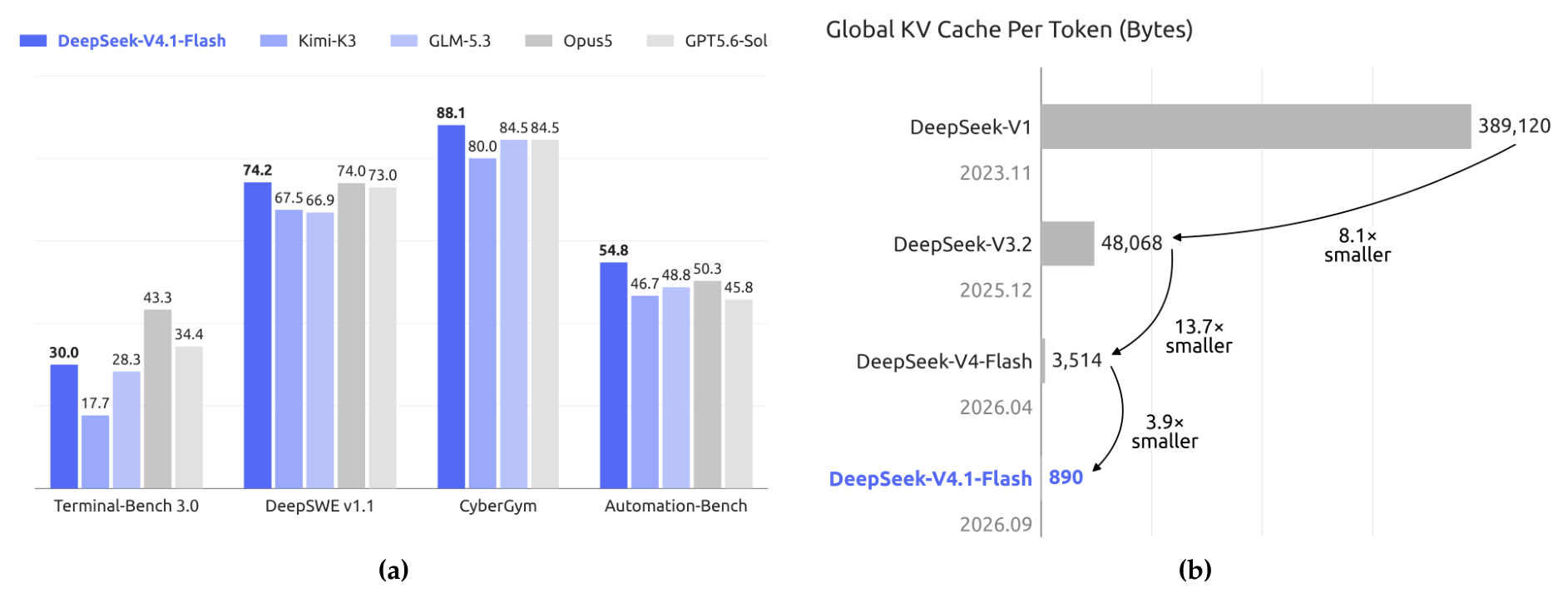
The two figures on the report's front page answer "how good" and "how cheap":
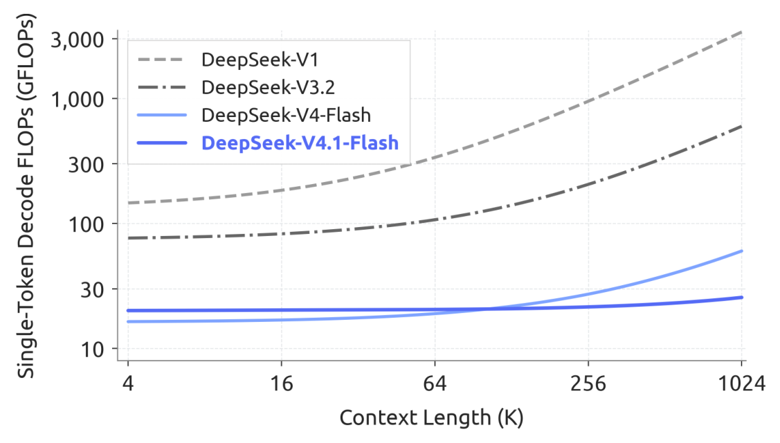
The second headline gain is "compute stays constant": thanks to sparse attention, speculative decoding, and friends, per-token decode compute barely grows with context length:
💡 Click any image to view the full-resolution original; click again or press Esc to close.
Background & Motivation: the Triple Bottleneck
With the explosion of agent applications, the workload shape changed: a single task calls tools repeatedly over hours, each round carrying a longer context. The report splits deployment cost into three ledgers:
- Compute: prefill on a KV-cache miss is expensive — sparse attention (DeepSeek-V3.2, V4) already cut long-sequence compute a lot, but prefill still dominates;
- Storage: global KV lives in HBM (capacity-bound); persistent KV for prefix reuse lands on SSD / host memory (capacity- and retention-bound);
- Bandwidth: cache migration and loading are limited by I/O and interconnect bandwidth, capping serving throughput.
DeepSeek-V4's attention mixes a global branch with per-layer sliding-window attention (SWA): the global branch keeps global KV (main KV + indexer K), SWA keeps local KV. With a fixed window, SWA storage is bounded, so for long enough sequences global KV dominates runtime footprint. Since V4 already pushed "compute" low enough, "store" and "move" became the new bottlenecks — exactly where V4.1-Flash aims.
The authors offer a crisp conceptual reframing: DeepSeek-V4 is essentially "an SWA local-processing backbone augmented with compressed global context." Following that view, V4.1's strategy is to leave the local SWA design alone and concentrate on simplifying the global branch. That yields three cooperating designs — CSA2 (share global KV and indices across layers), FP4 global KV (halve storage again), and SWA Bounded Replay (stop persisting SWA KV). The model also moves from V4's CSA+HCA hybrid to pure CSA2, simplifying further.
Architecture: a 40-Layer CED + Multimodal Pathway
DeepSeek-V4.1-Flash is a multimodal MoE Transformer: images and text in, text out autoregressively. The language backbone has 40 causal Transformer layers organized as "20-layer causal encoder + 20-layer decoder" — the CED structure; except for the first two layers (SWA only), every layer carries both global attention and sliding-window attention. On the vision side, a ViT encoder plus an MLP projector turn images into visual embeddings that are processed jointly with text — multimodal data is in the mix from the first day of pre-training.
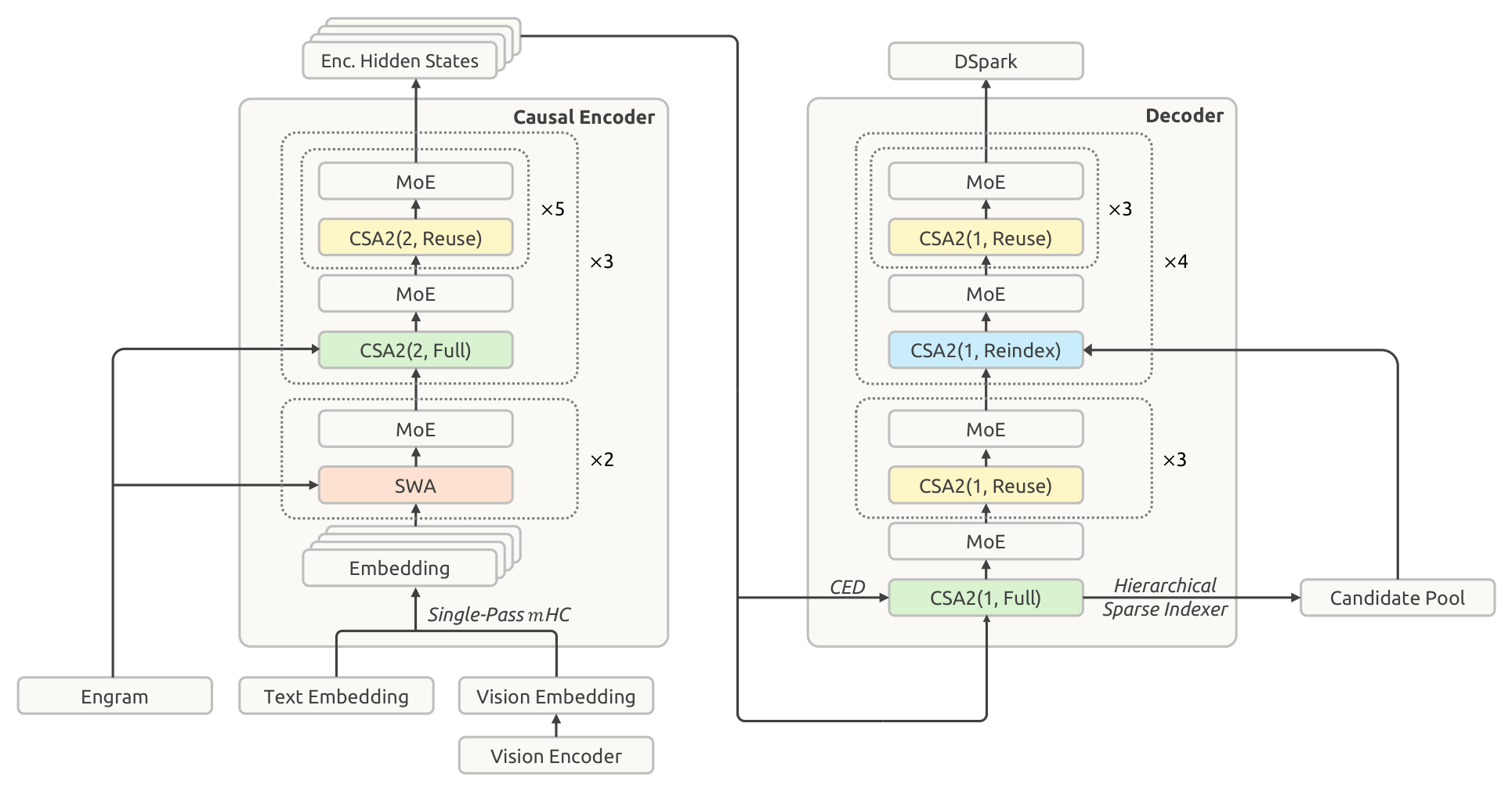
Key facts, itemized:
- Parameter ledger: 552B backbone + 196B Engram; 8B activated per token in prefill, 16B in decode — the asymmetric activation is a direct product of CED (next section);
- MoE configuration: DeepSeekMoE's shared + fine-grained routed experts; each layer has 1 shared expert + 384 routed experts, 6 activated per token, expert intermediate dimension 2304, SwiGLU activation clamped at 10;
- Attention configuration: indexer with 32 query heads, head dim 128, Top-512 KV entries selected per query; main attention with 64 query heads, head dim 512, query compression dimension 1280; SWA window $n_{\text{win}}=128$.
Multimodal architecture: DeepSeek-ViT and modality-specific load balancing
The vision pathway = ViT encoder + MLP projector. The ViT is trained from scratch with several changes to handle arbitrary resolutions: 2D-RoPE replaces absolute positional embeddings; the patch-embedding convolution becomes a linear projection (for Muon-optimizer compatibility); RMSNorm + SwiGLU throughout. Before features enter the LLM, a 3×3 pixel-unshuffle cuts spatial resolution by a factor of nine, effectively supporting inputs up to ~1344×1344 pixels. The ViT has 32 layers, hidden dim 1024, 16 attention heads, patch size 14; the projector has 2 layers with hidden dim 5120.
One MoE-side detail: modality-specific auxiliary-loss-free load balancing. Image and text tokens have different representation distributions and hence different expert-routing preferences; balancing them in aggregate would mask within-modality imbalance. So the model keeps separate expert-wise correction biases for text and image tokens: at routing time each modality uses its own biases for expert selection, while weighting still uses the original routing scores; after each training step the two bias sets update independently from their respective loads. A small change that makes multimodal training noticeably more stable.
Core Methods: CED and CSA2
CED: run only half the layers in prefill
Frequent tool calls in agent workflows generate massive prefill requests; whenever the KV cache misses, prefill cost bites. CED inherits the idea from YoCo ("You Only Cache Once"): let the upper half of the layers share the KV produced by the lower half. The difference is that CED adds two structural refinements — improving both the overall KV capacity and the computational depth of KV generation.
Concretely, for global attention the bottom $L/2$ layers act as the causal encoder; the decoder layers ($l > L/2$) no longer derive KV from their own hidden states $H_l$, but project it directly from the $L/2$-th (final encoder) hidden state $H_{L/2}$ with layer-dependent weights:
where $C_l$ is the KV entries and $Z_l$ the associated compression weights. Prefill then only has to fully compute the first half of the network, and the upper half's global KV arrives at the cost of a small projection — activated parameters per token drop from 16B (decode) to 8B (prefill). For input-heavy agentic loads, that is the most direct saving.
SWA keeps the conventional layer-wise computation: layer $l$'s local keys and values still come from its own hidden state $H_l$. This preserves the computational depth of local KV generation, but the price is a replay process in the decoder — computing decoder SWA KV during prefill needs an extra $n_{\text{win}} \times L/2$ tokens. For multi-turn interactions with short prompts per turn, that overhead is non-negligible. Hence Decoder SWA Bounded Replay: replay only the last $n_{\text{win}}$ tokens of the prompt for SWA (instead of $L \times n_{\text{win}}$).
Overall, for sequence length $N \gg n_{\text{win}}$:
prefill compute is roughly halved.
CSA2: compress along three dimensions at once
Serving long contexts means controlling both KV storage and attention compute. The report sorts existing techniques into three multiplicative dimensions:
- Entry dimension: GQA reduces KV heads; MLA shares a small latent across heads;
- Sequence dimension: every $m$ tokens compress into one entry (as in CSA/HCA);
- Layer dimension: some layers reuse other layers' caches or selections (IndexCache reuses indices only; YOIO computes routing once and shares network-wide; HySparse lets sparse layers reuse dense-layer KV).
The gap in prior work: reusing indices alone saves no main-KV storage; network-wide routing sharing caps performance; hybrid designs still keep full-attention layers — none of them covers all three dimensions at once. CSA2's answer is the joint attack: share main KV and indexer K across layers, allow Top-K index reuse, and decouple "cache sharing" from "index reuse". Two further simplifications versus CSA: drop the overlap between adjacent compressed entries and the absolute positional embedding; derive indexer K by projecting main KV (no separate compression path from hidden states) — both simplify implementation and speed up training.
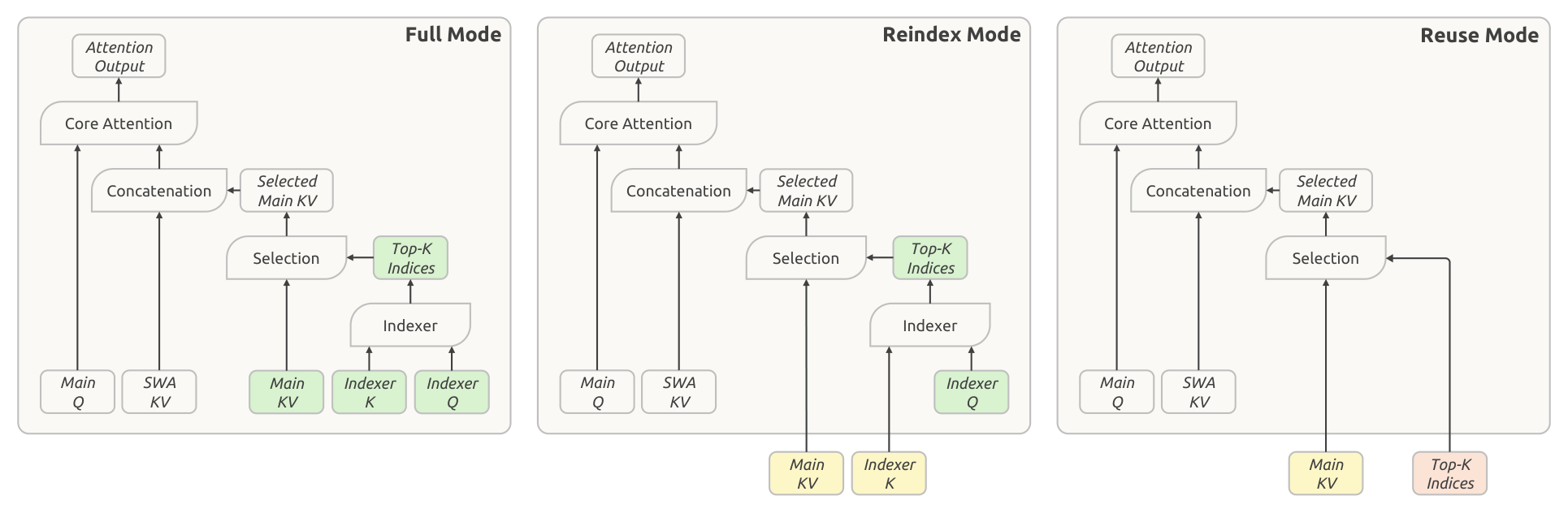
Modes and their responsibilities:
- Full Mode: computes its own main KV and indexer Q, projects indexer K from that main KV, runs the indexer for fresh Top-K indices — the complete CSA2 computation path;
- Reindex Mode: reuses the most recent available main KV and its indexer K, but rescoring with its own indexer Q produces new Top-K — cache shared, selection free to vary;
- Reuse Mode: reuses both main KV and Top-K indices, attends directly — no indexer Q, no index scoring.
Sharing main KV and indexer K removes duplicated storage; reusing Top-K indices removes index computation; Reindex mode keeps cache sharing while letting each layer select different entries. Under CED, the decoder's Full-Mode layers derive global KV from the final encoder hidden state; Reindex/Reuse are unchanged.
Hierarchical Sparse Indexer: making deep-indexer cost constant
Cross-layer index reuse cuts the number of indexer evaluations, but the surviving indexers still score the full causally visible context — at extreme lengths that remains a compute bottleneck. The Hierarchical Sparse Indexer (decoder-only under CED) rests on a simple observation: information from shallower indexers can naturally restrict the candidates considered by deeper ones, with zero extra state.
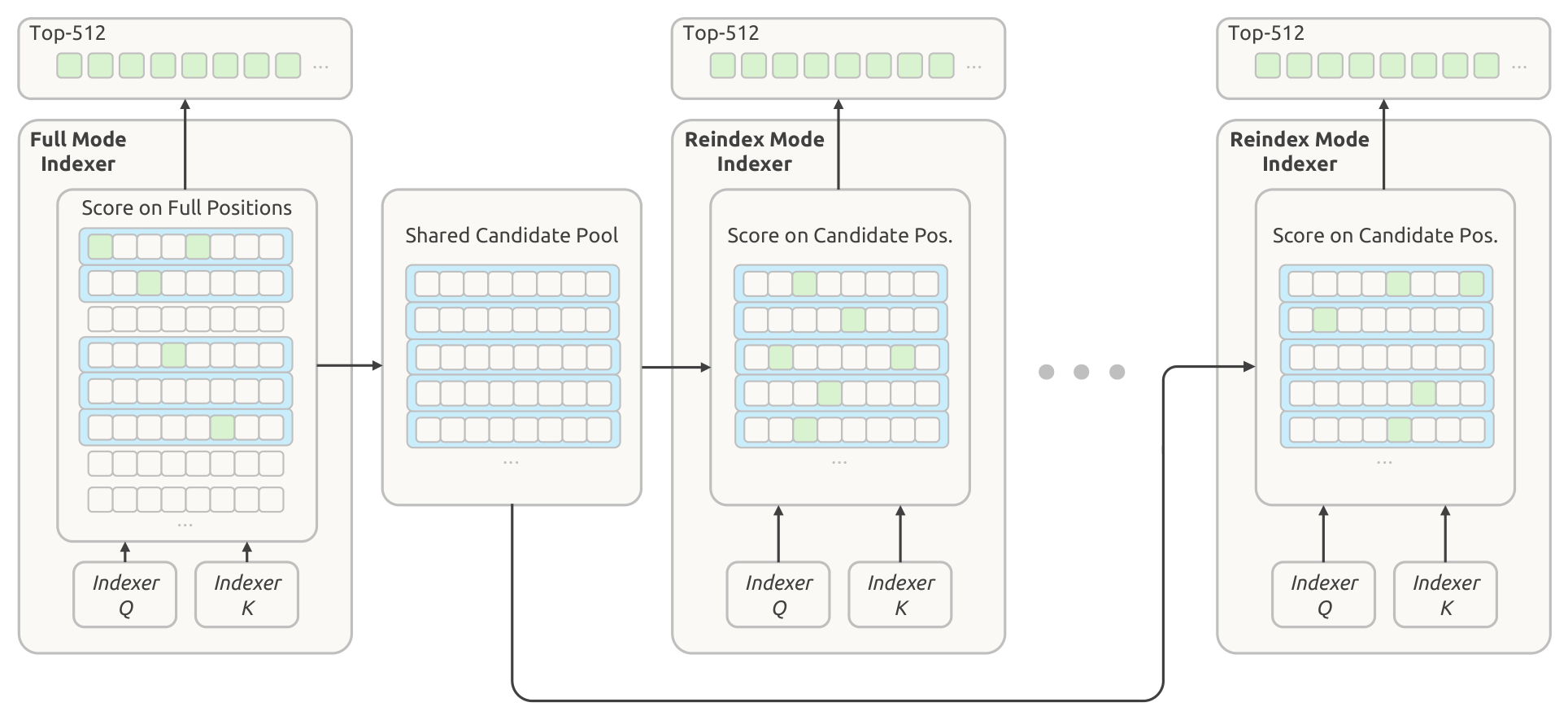
Mechanics: the first Full layer scans everything and builds the pool; the pool is much larger than the final Top-K (16,384 vs 512); subsequent Reindex layers search only inside it and pick different final entries, while Reuse layers do no indexing. The mechanism is training-aware: the candidate restriction is applied identically in training and inference, so deeper indexers are optimized under the same search domain they see at deployment. Per-query cost of deep indexers drops from "linear in context" to "constant" — the only price is the first layer's single full-range pass.
Efficient Extensions: mHC, Engram, DSpark, FP4, and Optimizers
Single-Pass mHC: halving activation memory traffic
mHC maintains $n$ residual streams between adjacent Transformer blocks, with per-token coefficients $A_l, B_l, C_l$ predicted from $X_l$:
Ideally the residual transformation between two blocks is a single map $(X_{l-1}, Y_{l-1}) \to (X_l, \hat{X}_l)$ with a lower bound of $(2n+2)d$ on activation traffic. But DeepSeek-V4's three-kernel implementation realizes $(4n+4)d$ — exactly twice the bound. The culprit is a dependency: input mixing $\hat{X}_l = A_l X_l$ must wait for the full reduction over $X_l$ (to produce $A_l$), forcing a second read of $X_l$.
Single-Pass mHC's fix is elegant: shift the input-mixing coefficients by one block — each block consumes the coefficients produced by the previous one:
With the dependency gone, each tile of $X_l$ can simultaneously drive input mixing and accumulate the projection outputs and sums of squares needed for coefficient prediction. Pre-training keeps the multi-kernel implementation (only the coefficient provenance changes); at deployment, residual update, input mixing, coefficient prediction, pre-norm, and FP8 conversion all fuse into a single Mega-mHC kernel, bringing activation traffic to $(2n+2)d$ — exactly the lower bound, half of the original. Empirically the shift costs almost nothing.
Engram: 196B parameters of conditional memory
Engram decouples "memory" from computation: tokenizer compression, multi-head hashing, context-aware gating, and multi-branch integration. V4.1-Flash makes two changes: drop the short causal convolution (gains didn't justify inference-stack complexity), and optimize the embedding tables with momentum + Sinkhorn balancing (below). Configuration: 196B parameters split evenly across two modules at layers 1 and 14 (for pipeline memory balance); $N$-gram orders {2, 3, 4}, 8 hash heads, total embedding dimension 2048 per order; each head indexes a table of ~16M entries with distinct prime sizes; embedding tables and K/V projections in FP8. At inference, deterministic addressing lets embeddings be prefetched from host memory via background RDMA — the first module's prefetch overlaps the first Transformer block's compute.
DSpark: confidence-scheduled speculative decoding
DSpark = semi-autoregressive drafting + confidence-scheduled verification. The drafter is 3 Transformer blocks (128-token sliding window); a single forward pass computes base logits for 5 draft positions in parallel, a lightweight Markov head models dependencies among draft tokens, and a confidence head predicts per-position conditional acceptance probabilities to estimate prefix survival probabilities. The scheduler combines these estimates with profiled engine-throughput curves to pick a per-request verification length that maximizes expected system-wide token throughput under current load. Unlike DeepSeek-V3's MTP, DSpark is trained in a dedicated stage after backbone pre-training (backbone frozen); during post-training it trains alongside the backbone without propagating its gradients into it — staying aligned with the evolving policy while accelerating both online serving and RL/OPD rollouts.
FP4 main KV cache: E2M1 with one E4M3 scale per 16 channels
V4 already applied QAT to indexer Q/K to accelerate indexing; V4.1 extends QAT to the main KV — note that FP4 here is for storage, not faster matmuls: values are dequantized before attention, so no native FP4 matmul hardware is needed and portability is preserved. The format is OCP-standard MXFP4 (even though alternatives scored slightly higher in tests): E2M1 with one E4M3 scale per 16 channels; following NVFP4 but omitting the second-level global scale. The feasibility argument is neat: after RMSNorm the 512-channel KV latent has L2 norm at most $\sqrt{512} \approx 22.6$ (largest trained RMSNorm weight ≈ 1, RoPE preserves norms), while the format supports magnitudes up to $448 \times 6 = 2688$ and training observed maxima around 10 — dropping the global scale causes no measurable accuracy loss and simplifies the cache layout. Implementation details: quantize after RoPE (quantizing before gave only marginal gains and would add decode-time overhead); non-RoPE and RoPE components share the format; QAT enters during post-training; SWA KV stays FP8 (quantization-sensitive). Versus V4's FP8 main KV, storage halves again — in HBM and on SSD alike.
Optimizers: head-wise Muon + Sinkhorn-balanced updates
The base configuration continues V4: AdamW for normalization-layer and other non-matrix parameters ($\beta_1=0.9$, $\beta_2=0.95$, $\varepsilon=10^{-20}$, weight decay 0.1); Muon for linear-transformation weights (including Engram projections and the vision-language projector) with momentum 0.95, decoupled weight decay, and Nesterov momentum, rescaling each update's RMS to 0.18 to reuse the AdamW learning rate. Two new designs:
- Head-wise Muon: split the Query (and Key) weights by head before the Muon update. Viewing Muon as preconditioned gradient descent, vanilla Muon shares one preconditioner across all heads, yet attention heads are heterogeneous — grouping by head empirically beats vanilla (independently corroborated by GLM-5 and Kimi-K3);
- Sinkhorn-balanced update: applying Adam to the newly added Engram parameters would blow up optimizer-state memory. Instead: momentum + Sinkhorn balancing — same skeleton as Muon, but Newton–Schulz orthogonalization is replaced by alternating row/column normalization. It needs only a momentum buffer and empirically outperforms Adam.
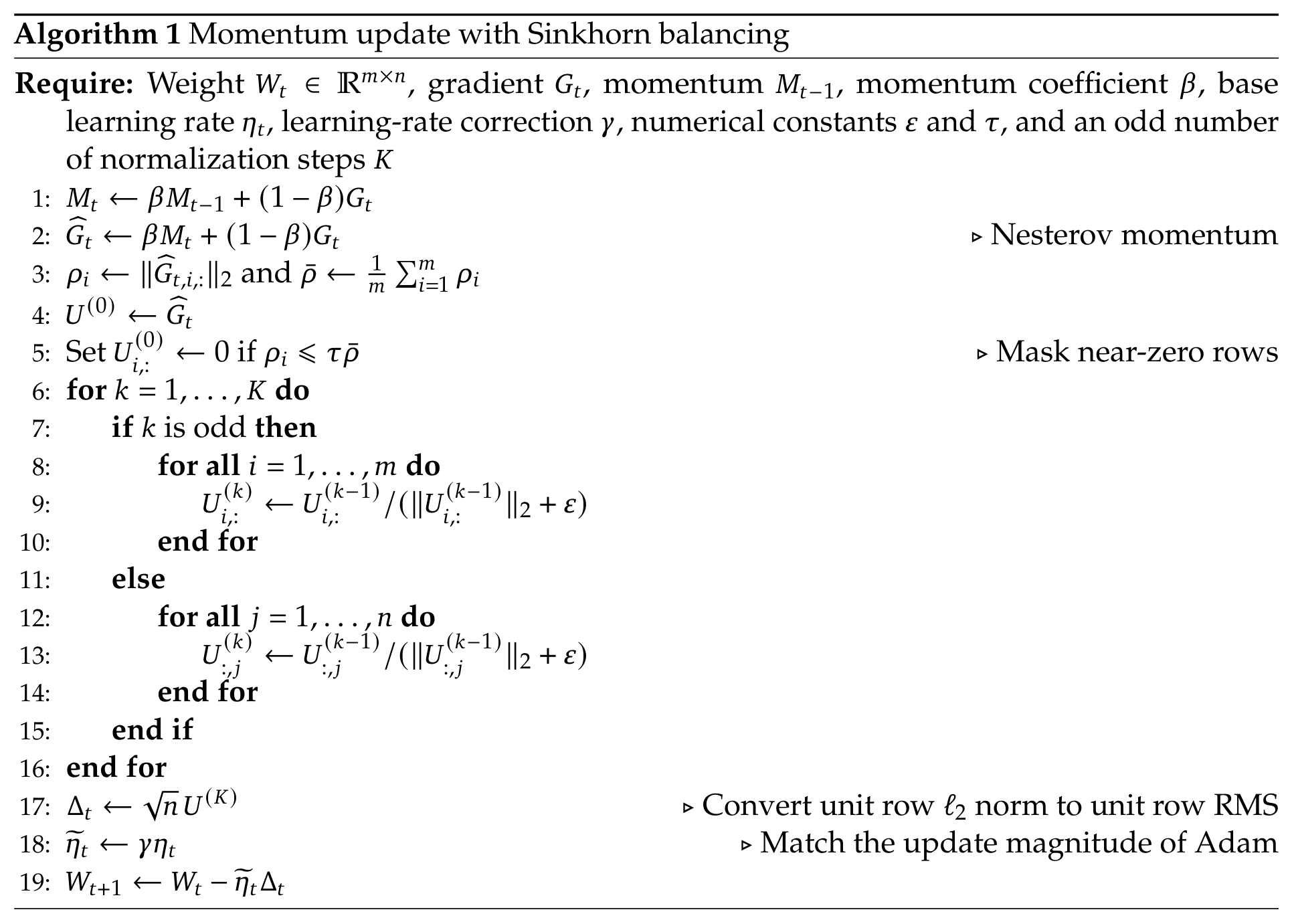
In the training configuration the Sinkhorn update uses $K=11$, $\tau=10^{-3}$, $\varepsilon=10^{-20}$, with momentum and learning-rate correction matching Muon; the Engram learning rate is scaled 5×. The authors also situate the update among axis-structure-aware optimizers (Adafactor, Adam-mini, SRON, etc.), leaving finer comparisons to future work.
Infrastructure: Training and Inference Systems
For the architectural gains to materialize, the training and inference systems must be co-designed with the architecture. The report's principle: the architecture may be intricate, but the kernel flow must be remarkably concise.
Training infrastructure: three pieces
① Multimodal training: disaggregated encoder and hidden communication
The vision encoder is first optimized with a contrastive objective, then fine-tuned with a generative next-token loss. The contrastive phase computes the loss over a full batch of text-vision pairs, so features of both modalities must be all-gathered across data-parallel ranks — substantial communication. The key observation: the gradient of the text features depends only on the gathered visual features (and symmetrically for visual features), so both all-gathers can hide entirely behind compute:
For end-to-end parallelism, the disaggregated-encoder design places the ViT outside the LLM parameter tree; each training step runs in three phases — vision-encoder forward, LLM forward/backward, vision-encoder backward — so vision load is confined to the first and last phases and the LLM phase keeps the parallel strategy of text-only training. Ultra-long multimodal training adds two optimizations: balanced image sharding (each sequence's images are sharded across CP ranks with load balancing, each image read exactly once; the criterion involves only per-token quantities — whenever $\rho < B_{\text{IO}}/(B_{\text{GPU}} C)$, loading hides behind compute regardless of sequence length or cluster size) and incremental image transfer (RL rollouts send only deltas, with CPU-side decoding and preprocessing cached on a distributed filesystem for reuse).
② Training with shared attention states (CSA2)
Layers that share attention components may sit on different pipeline stages, so direct module reuse is incompatible with stage-local execution. Three mechanisms resolve this:
- Shadow indexers: each participating stage holds a lightweight executable replica while a single logical owner keeps the shared parameters (optimization and checkpointing); parameter synchronization and gradient aggregation keep replicas consistent — the pipeline scheduler never treats shared layers as a special unit;
- Pipeline payload extensions: when producers and consumers straddle a stage boundary, the intermediate representations and sparse-routing information ride the existing point-to-point communication path, partitioned consistently with context parallelism;
- Micro-batch-level shared-state management: tracks the states of concurrently active micro-batches across forward, activation recomputation, and backward, releasing each state promptly after its final consumer finishes.
③ Engram parallelism
Embedding tables are partitioned by row across dedicated process groups (the engram-parallel size trades per-device memory against lookup communication scope); optimizer states are further sharded across replicas. Embedding prefetch fires for the whole local batch before each pipeline stage begins; embedding gradients are buffered during backward and returned to their owning ranks after the backbone backward; both overlap the vision encoder's forward/backward. Embeddings are stored and fetched in FP8, with retrieved values and scaling factors fed straight into the following GEMM. During RL rollouts the tables stay resident in GPU memory, avoiding host-memory-fragmentation OOMs.
Inference system: few kernels, EPD disaggregation, and a persistent-cache overhaul
Through kernel fusion (FlashMLA's fused RoPE-attention-RoPE-cast kernel, DeepGEMM's Mega-Gate/Mega-mHC/Mega-MoE, TileKernels, DeepSelect's TopK), the vast majority of Transformer layers — those whose CSA2 runs in Reuse Mode — execute with just 15 kernels in prefill and 11 in decode. Deployment uses EPD: vision encoding, prefill, and decoding scale independently and overlap.
Persistent KV cache management: evicting SWA KV from SSD
In the V4 deployment, SWA KV accounts for nearly half of persistent-cache capacity: global and SWA KV are managed independently under LRU; SWA KV is cached only at two points (end of prompt, end of output), yet even retaining only $n_{\text{win}}$ entries per point, uncompressed storage is costly — and the 72-hour retention policy fundamentally mismatches SWA's minute-scale reuse window: once a session ends, the data is dead. V4's proposed Zero SWA Caching recovered misses by full recomputation over $L \times n_{\text{win}}$ tokens — too expensive for production.
V4.1's revision settles the matter:
- SWA KV leaves the persistent cache entirely, moving into a distributed memory pool provisioned from 10% of host DRAM per machine. The pool is far smaller, but its TTL is minutes and expired entries recycle immediately for new sessions — the turnover suffices for the vast majority of concurrent active sessions; global KV remains persistent with a guaranteed ≥72-hour lifetime;
- A miss is no longer scary: Encoder SWA Bounded Replay is the lightweight fallback that turns a catastrophic miss into a graceful, inexpensive degradation — the cornerstone that justifies removing SWA KV from the persistent cache in the first place.
SWA Bounded Replay: one policy, two uses
SWA dependencies accumulate across layers; exactly reconstructing the SWA KV of $L$ layers requires replaying $L \times n_{\text{win}}$ tokens. Bounded Replay replays only the most recent $n_{\text{win}}$ tokens and truncates SWA to the replay segment: for a replay starting at position $s$, a query at position $i$ attends to SWA keys in $\left[\max(s, i-W+1),\, i\right]$ — approximate states accepted.
- Encoder SWA Bounded Replay makes prefix caching depend only on global KV. When encoder SWA KV is missing, the last $n_{\text{win}}$ tokens of the cached prefix are replayed and processed together with the uncached suffix; replayed tokens regenerate only SWA KV while the cached global KV is reused untouched. By design the replayed prefix state is approximate, so the KV computed for the suffix is not mathematically identical to the exact version — yet experiments show the response quality barely moves;
- Decoder SWA Bounded Replay bounds the decoder forward to $n_{\text{win}}$ tokens, nearly halving total prefill compute. Under CED the decoder's global KV is projected from the encoder's final state; the only obstacle is decoder SWA KV (generated per-layer, needed by the first decode steps). Since decoder SWA KV is never cached, exact reconstruction would run $L/2$ decoder layers over $L/2 \times n_{\text{win}}$ prompt tokens — expensive precisely when a long cached prefix meets a short uncached suffix. So every prefill replays the last $n_{\text{win}}$ prompt tokens, feeds their encoder outputs through the decoder layers under the same SWA truncation, and uses the resulting SWA KV for decoding only — never for prefix caching. For extra safety, post-training simulates the same replay for train-aware adaptation.
Pre-Training: 45T Multimodal Tokens and Evaluation
Data construction: from sample quality to corpus-level interactions
On the text side, this generation's pipeline shifts focus from the "sample-level quality reflected by small-scale experiments" to holistic interactions and information gains across diverse corpora: a scaling ladder over model parameters and training data guides large-scale runs; model-generated content with limited information gain (weaker-model outputs, low-quality machine translation) is filtered out — treated as implicit duplication that becomes detrimental over long horizons; more domain experts contribute fine-grained quality dimensions; and fresher code from newly released repositories, commits, libraries, and frameworks broadens language and real-world coverage.
The multimodal philosophy is "clean in native form, refuse large-scale synthesis": raw web data naturally carries multimodal knowledge, so the pipeline prioritizes cleaning and using it natively. The crawler was re-bootstrapped from Common Crawl (it had skewed text-centric); image-text pairs are filtered by image-text relevance thresholds and deduplicated by image semantics; interleaved data comes mainly from webpages and PDFs, processed in progressively more expensive stages (heuristic/statistical filtering, dedup, quality models first; image-aware filtering and dedup next; strict SmolVLM quality scoring last), with filtered-out documents partly recycled into extra image-text pairs; domain-specific data supplements fine-grained perception (grounding/pointing), OCR, and long-tail knowledge, plus image-code pairs and computer-use trajectories. The final corpus merges at a 7 : 1 text-only : multimodal token ratio (overlapping samples replaced by their multimodal versions), ultra-long documents are deterministically pre-split, and an improved best-fit packing keeps the padding rate at most $10^{-4}$.
Training setup: sparse from scratch, starting at 64K
- Model configuration: 40 layers, hidden dim 5120; first 2 layers pure SWA; 18 encoder CSA2 layers (ratio $m=2$) in 3 groups of 6 (1 Full + 5 Reuse); 20 decoder CSA2 layers ($m=1$) in 5 groups of 4 (first group 1 Full + 3 Reuse, the rest 1 Reindex + 3 Reuse); hierarchical indexer with 2,048 blocks × 8 positions = 16,384 candidates; 8 output-projection groups, intermediate attention-output dim 1024;
- Training recipe: 45T tokens with no instability; batch fixed at 100.6M tokens; learning rate warms linearly over the first 2000 steps, holds at $2.6\times10^{-4}$ until 28T, cosine-decays to $2.6\times10^{-5}$ between 28T and 40T, then holds to 45T; sparse attention trained from scratch at 64K (no dense-attention warmup), extended to 1M at 34T; auxiliary-loss-free balancing with bias update speed 0.001 per modality plus a small sequence-level balance loss (weight 0.0001); sample-level attention masking continues from V4;
- Two-stage ViT training: contrastive pre-training with SigLIP's sigmoid loss on ~47B image-text pairs at 224×224 (higher resolutions add little here); autoregressive fine-tuning with a 4B MoE LLM on 236B tokens (resolution 544×544 to 1344×1344), after which the LLM is discarded and only the optimized vision encoder enters main pre-training.
Base-model evaluation: Pro-level results at 1/3 the parameters
The base comparison spans world knowledge, language understanding & reasoning, coding & math, long context, and multimodality:
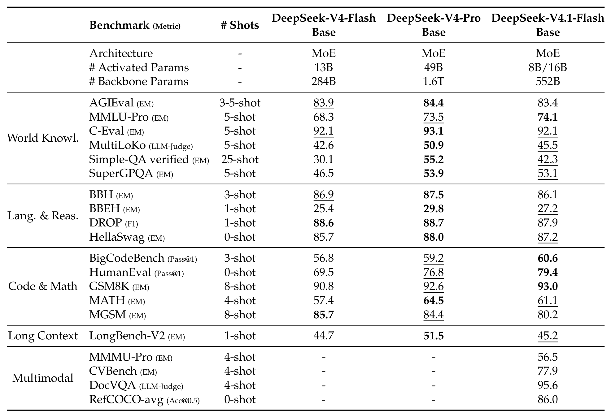
By category: world knowledge and language understanding land in the same band (MMLU-Pro 74.1 above Pro's 73.5; BBH/BBEH/DROP within 0.3–2.7); coding and math lead on several rows (BigCodeBench 60.6, HumanEval 79.4, GSM8K 93.0); MGSM at 80.2 is the notable regression (below Flash's 85.7 and Pro's 84.4); LongBench-V2 at 45.2 matches Flash and trails Pro's 51.5. The report credits the data pipeline's quality improvements as well.
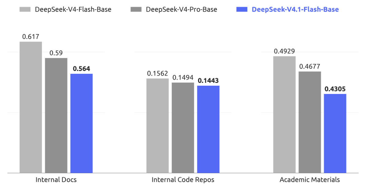
Real competence beyond APIs shows in perplexity. The team ran bits-per-byte (lower is better) tests on held-out internal corpora (internal documentation, proprietary code repositories, academic materials):
Post-Training: No New Algorithms, Just Data and Scale
This release deliberately introduces no post-training algorithms: the recipe is the standard SFT → RL → OPD, unmodified beyond well-established DeepSeek-V4 practice. All the investment goes into "what to train on" rather than "how to optimize" — large-scale, automated pipelines for task synthesis and environment construction. The authors' one-line conclusion is blunt: under a fixed, unremarkable optimization procedure, improvements in the scale, diversity, and verifiability of synthesized data and environments account for essentially all the gains; at this stage, the marginal return of engineering the data pipeline far exceeds that of algorithmic novelty.
Large-scale agent task synthesis
Each task is formalized as a triplet (problem, environment, verification system), evaluated along difficulty (non-trivial) and correctness (no critical flaws among the three components); both serve as reward signals to iteratively train the model to construct better tasks, and every reuse of a task in a new RL run yields fresh trajectories for quality re-auditing. Two dedicated pipelines:
- General agents: employees and external partners are encouraged to fold the latest model into daily workflows and voluntarily return interaction data; from the observed interfaces the team builds a large set of mocked tools faithfully reproducing real SaaS/enterprise systems — input formats, output structures, API schemas, behavioral constraints. Negative feedback and failure cases are collected at scale, and the pipeline reconstructs tool context, user-interaction patterns, and failure conditions for systematic failure replay and targeted RL;
- Coding agents: environments come from internal/partner coding sessions (keeping highly complex or poorly-performing tasks, deduplicated by trajectory) and public GitHub repos above a star threshold. Construction is multi-agent: one agent checks whether the project builds, runs, and auto-verifies inside a container, picks a commit/turn as the starting point, designs several sufficiently complex implementation directions, and produces fail-to-pass / pass-to-pass evaluation points; another agent sets up dependencies, the initial working directory, test code, and task descriptions in an isolated container, self-tests, scrubs any solution-leaking traces, and packages the environment as a new image layer; then several distinct agents attempt the task while an independent quality-inspection agent reviews environment and trajectories (environment defects, factual errors, evaluation-point mismatches, hackability); failed inspections go to a repair agent and re-verification.
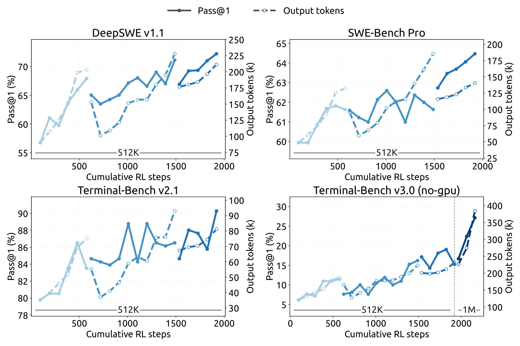
Scaling RL: compute and scaffolds
Large-scale asynchronous RL on synthesized tasks scales along two axes: training compute and the number of scaffolds. Rollout execution is decoupled into an agent sandbox + worker container: the sandbox runs the scaffold and its tools; the worker provides a scaffold-agnostic control layer (orchestrating rollouts, normalizing heterogeneous interactions into a common trajectory schema, talking to the trainer). Both run on DSec, outside the preemptible GPU training pool; on trainer preemption, rollouts suspend with full state and resume later. Successive RL runs are reinitialized via model merging, combining improvements acquired along different optimization paths and continuing to scale.
DSec: elastic compute for millions of sandboxes
From V3 to V4, the exploding number and diversity of agentic environments motivated DeepSeek Elastic Compute (DSec), a production-grade sandbox platform. V4.1 pushed demand to millions of concurrent sandbox instances, shifting the bottlenecks to datacenter scalability, workload isolation, per-node compute density, and containing increasingly capable misbehaving agents:
- Horizontal scaling: sharding (scale units) isolates experiments and contains blast radius; instead of Kubernetes, a custom placement engine trades strong global consistency for scalability — multiple independent replicas make good-enough placements from recent measurements, with each node enforcing a hard local admission check. The system scales to millions of containers without a central-coordination bottleneck;
- High density: hardware sub-NUMA partitioning binds each worker VM to its own NUMA domain with containers confined to local NUMA resources — under comparable workloads, concurrent live containers per physical node rise from ~1,000 to 2,500+ before measurable end-to-end degradation. A latency-sensitive (LS) execution class applies SCHED_IDLE to non-LS tasks, and core scheduling keeps sibling hyperthreads to same-priority tasks, eliminating evaluation interference;
- Containing misbehaving agents: during RL, agents attempt reward hacking or crash environments — documented exploits include the XFS-driver permission issue, illegal memory access in AppArmor, answer leaks from package-mirror services, plus deleting critical binaries, breaking system files, or removing the filesystem. Countermeasures: per-sandbox AppArmor profiles and fine-grained eBPF network policies; a crashed environment counts as a failed trajectory with a "repercussion" signal to the RL framework.
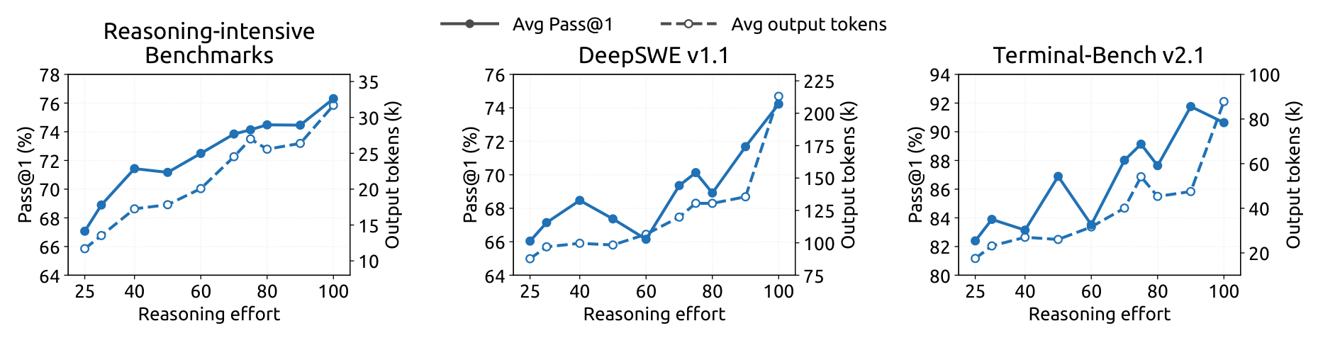
Controllable reasoning effort: one scalar for the cost-quality frontier
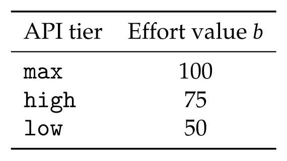
Beyond architecture and hardware, output-token count is the other determinant of serving cost. V4.1 introduces a scalar effort level $b \in \{1,\dots,100\}$ as an explicit conditioning signal prepended to the system prompt ("Reasoning Effort: {effort}; higher values request more thorough reasoning"), applied to both single-turn reasoning and multi-turn agentic tasks. For each training prompt, $M_b$ responses are sampled per effort level; rewards are mean-centered within each $(x, b)$ subgroup (effort levels are never directly compared); effort-dependent behavior is induced by the length component of the reward:
with $\ell_{b,j}$ the reasoning-token count, $L_{\text{norm}}$ a reference length, and $C_{\max}$ the deduction cap; the token-penalty coefficient decays exponentially — each increment of $b$ by $\tau$ multiplies the coefficient by $e^{-1}$. $k_0$ sets the overall pressure toward brevity; smaller $\tau$ separates effort levels more sharply. Appendix C derives the exponential parameterization from marginal utility: if the marginal solve-probability decays roughly as $p'_x(\ell) \approx a_x e^{-\ell/s_x}$, the preferred reasoning length is approximately affine in $b$:
At deployment, $b$ becomes a continuous dial over reasoning strength on a single checkpoint — intermediate values never seen in training interpolate smoothly. The public API (launched September 2026) exposes three preset tiers:
Asynchronous post-training infrastructure
The long-tail problem in RL rollouts (a few stragglers stalling every batch) is the classic efficiency killer. V4.1 made the post-training infrastructure end-to-end asynchronous, covering nearly all RL and OPD tasks:
- Sample-level dispatch: rollout and training colocate and time-share the same devices; each task caps in-flight samples. Three dispatch granularities were tried — batch-level (metrics oscillated badly, too coarse), prompt-level (stalls easily on long-tail samples inside a GRPO group), and finally sample-level: dispatch a prompt as soon as enough new samples arrive to fill its GRPO group, keeping concurrency flat throughout;
- Two side effects, two handles each: length-distribution bias (short sequences finish first and dominate early batches) — per-dataset concurrency limits plus discarding early-returned short samples to smooth the transition; off-policy drift (samples partially or wholly from older checkpoints) — dispatching/waiting logic bounds the maximum off-policy ratio, and a loss-masking scheme drops excessively stale tokens;
- Seamless switching: once enough training samples accumulate, training preempts rollouts with token-level interruption; KV cache and expert routing persist at token granularity so resumption with a new checkpoint continues exactly where things stopped, no re-prefill; sample-grained GC frees each sample's states upon completion; samples spanning checkpoints use concatenated routing-replay. The same machinery also lets training jobs yield to cluster preemption without losing progress;
- Large-scale OPD: the final full-vocabulary OPD spans all domains with 40+ teachers (the best teacher per domain may come from a different development stage, with heterogeneous architectures); the infrastructure supports near-zero-cost switching among architecturally heterogeneous teachers and consistent dynamic reconfiguration of dataset mixtures, per-dataset concurrency caps, and active teachers under asynchrony.
Evaluation: agent capability aligned with the closed-source frontier
Post-training evaluation focuses on reasoning and agency (knowledge is largely settled by pre-training; see Table 1). Reasoning: GPQA Diamond, HLE, Codeforces (internal benchmark), MathArena Apex at temperature/top-p 1.0. Agents fall into four categories: code agents, cyber security, general agents, and visual agents. Anti-reward-hacking measures: no internet, stripped Git histories, automatic purging of build/package caches — and exploits still surfaced (decompiling core Ubuntu packages to find vulnerabilities in CyberGym), prompting the authors to urge the community to prioritize detection and mitigation when designing next-generation benchmarks.
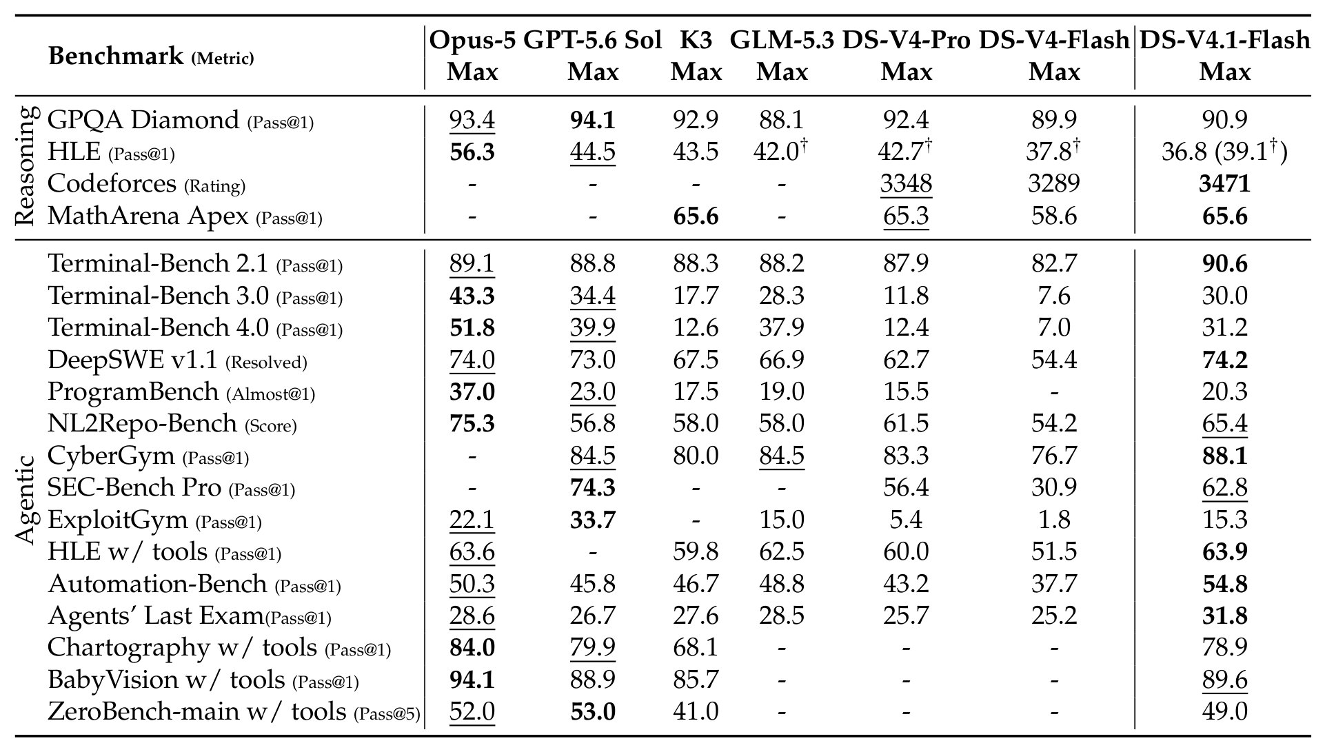
On cyber-security tasks V4.1-Flash sets a new open-source record — and the report explicitly flags the dual-use nature, encouraging responsible applications such as defensive security research and vulnerability remediation. Visual agents (Chartography 78.9, BabyVision 89.6, ZeroBench 49.0) beat the strongest open-source competitor Kimi-K3, though a measurable gap to the closed-source leaders remains.
Reasoning effort: one smooth cost-quality curve
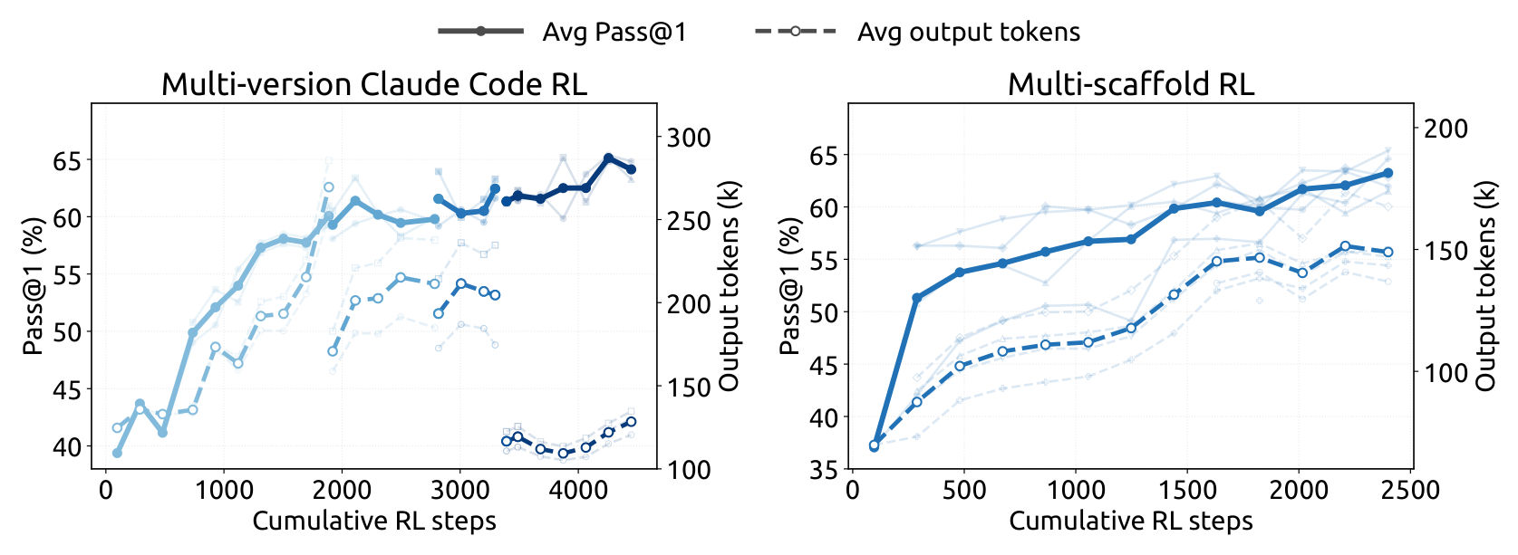
Cross-scaffold robustness: capability that doesn't pick its harness
In practice a model is rarely welded to one agent framework. The evaluation covers 8 configurations from 6 scaffold families (Claude Code, Codex, OpenCode, Pi, mini-SWE, DeepSeek Harness Minimal/Standard/PTC), changing only the harness while keeping the model and decoding fixed:


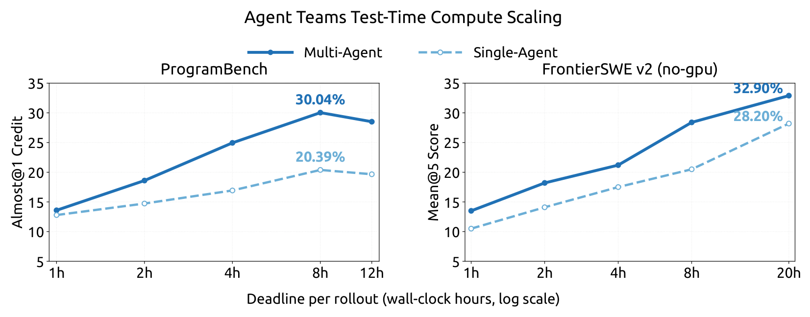
Multi-agent: first experiments with Agent Team mode
DeepSeek Harness's Agent Team mode explores multi-agent collaboration: a lead agent asynchronously creates named persistent teammates via spawn_teammate (fresh mode without lead history, or fork mode with a one-time snapshot of the lead's completed turns); all agents share one repository checkout so edits are immediately visible; a durable peer mailbox delivers messages at the next step boundary, starts new turns for idle teammates, or resumes inactive ones; a shared task board maintains ownership, dependencies, and advisory write scopes (updates with revision checks); when needed, only the lead can interrupt a teammate's turn via interrupt_agent. The training reward = task performance + a collaboration bonus (encouraging delegation and inter-agent communication) + a derived-latency penalty: execution events and their collaboration dependencies form a DAG, costs come from token counts at fixed prefill/decode rates plus measured tool-execution time, and the penalty is the critical-path length — rewarding useful parallelism, punishing needless serialization and synchronization, and staying insensitive to serving-side batching and queuing delays.
Evaluation uses a high-confidence ProgramBench subset (only tasks where the reference solution passes ≥95% on the hidden test suite — 172 "golden" tasks) and a no-GPU subset of FrontierSWE v2:
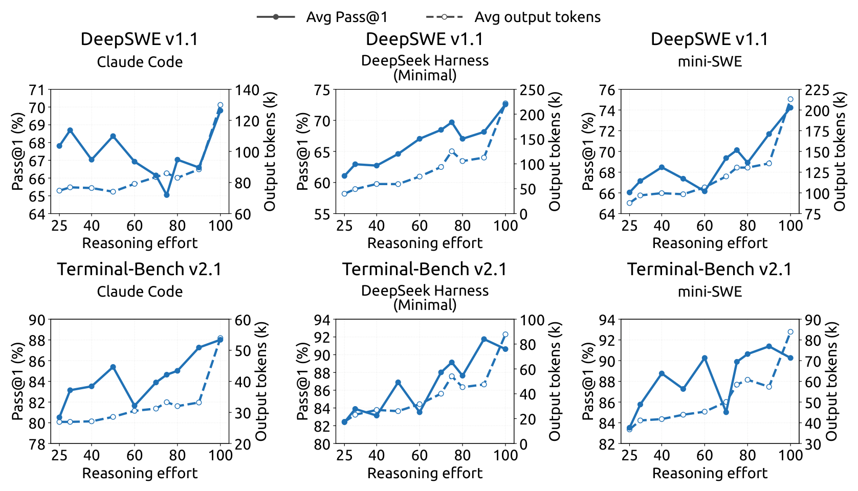
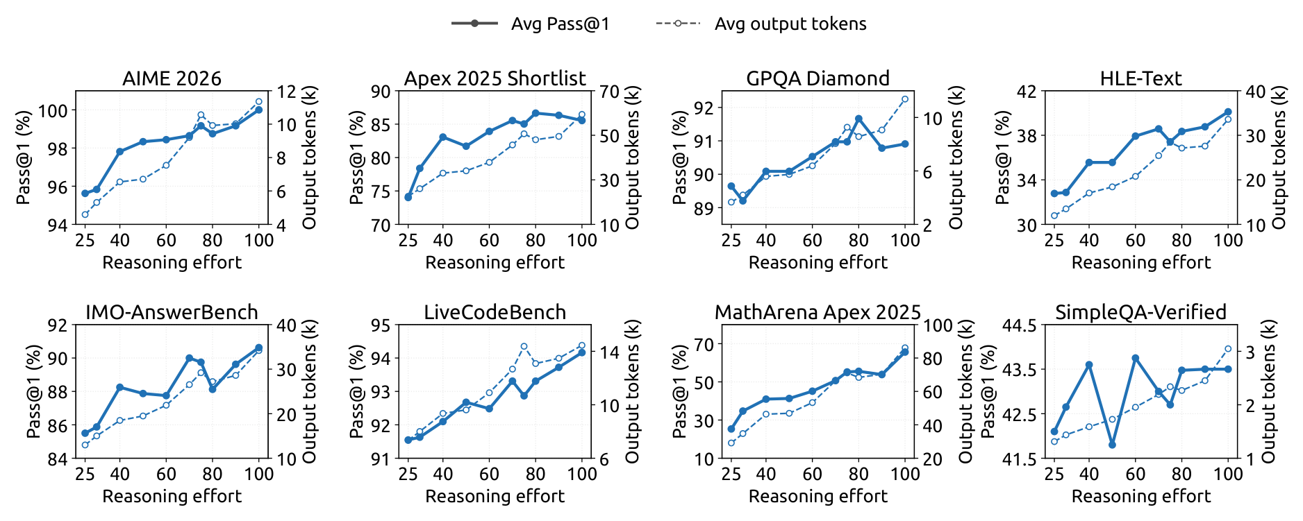
Appendix extras: fine-grained behavior of effort control across scaffolds and benchmarks
Glossary
Refer back here any time; dotted-underlined abbreviations in the text show their meaning on hover.
| Abbreviation | Full name | One-line explanation |
|---|---|---|
| MoE | Mixture-of-Experts | Each token activates only a few experts: huge total parameters, small activated set |
| CED | Causal Encoder-Decoder | Bottom half as encoder; upper layers' KV projected from the encoder's final state — prefill compute roughly halved |
| CSA2 | Compressed Sparse Attention 2 | Second-gen compressed sparse attention: cross-layer main-KV/indexer-K sharing with Top-K index reuse, in Full/Reindex/Reuse modes |
| SWA | Sliding-Window Attention | Each layer attends to the most recent n_win=128 tokens; storage bounded |
| KV Cache | Key-Value Cache | Attention's key-value cache — the dominant memory cost of long-context deployment |
| MLA / GQA | Multi-head Latent / Grouped-Query Attention | Two entry-dimension compression routes: shared latent across heads / fewer KV heads |
| HSI | Hierarchical Sparse Indexer | Decoder-only: first Full layer builds a 16,384-position candidate pool; deeper indexers cost O(1) |
| mHC | Manifold-constrained Hyper-Connections | Multi-stream residual mixing; Single-Pass shifts mixing coefficients one block back for a single-kernel, lower-bound implementation |
| QAT | Quantization-Aware Training | Simulate quantization during training to preserve accuracy at FP4/FP8 |
| MXFP4 | Microscaling FP4 (OCP) | OCP block-scaled FP4; here E2M1 with one E4M3 scale per 16 channels |
| EPD | Encoder-Prefill-Decode | Serving disaggregation: vision encoding, prefill, and decoding scale independently and overlap |
| SWA Bounded Replay | — | Replay only the last n_win tokens to approximately rebuild SWA KV: no SWA persistence, prefill halved again |
| DSec | DeepSeek Elastic Compute | Million-scale sandbox platform: sharding + relaxed-consistency scheduling + high-density NUMA isolation |
| OPD | On-Policy Distillation | Student samples, teacher supervises over the full vocabulary; the final post-training stage |
| SFT / RL | Supervised Fine-Tuning / Reinforcement Learning | The standard two post-training stages |
| DSH | DeepSeek Harness | DeepSeek's own agent framework with Minimal/Standard/PTC/Agent Team modes |
| BPB | Bits-Per-Byte | Per-byte bit count (a perplexity transform); lower compresses the corpus better |
| HLE / ALE | Humanity's Last Exam / Agents' Last Exam | Two "last exams": the ceiling of human knowledge / the ceiling of agent capability |
Commentary & Outlook
The paper's own conclusions and candid limitations
The authors' summary: through joint optimization of architecture, cache precision, and deployment strategy, V4.1-Flash pushes KV cache compression to new limits — 890 bytes/token global KV (≈1/4 of V4-Flash), persistent cache ≈1/8 — with an activation footprint far smaller than open-source peers like GLM-5.3 and Kimi-K3 while performing comparably or better on key benchmarks. The limitations are stated plainly:
- Robustness boundaries not fully characterized: CSA2 selection errors and Bounded Replay's approximate reconstruction could degrade capability on untested extreme inputs and deployment conditions; internal evaluations saw no systematic degradation, but no finite test suite covers everything — stress testing will continue (focus: sparse retrieval over long contexts and SWA reconstruction at cache-resumption boundaries);
- Benchmark saturation vs the real frontier: scores close to Fable-5 and GPT-6 Astra do not imply parity with closed-source frontiers on the hardest tasks and edge cases; evaluation protocols will keep evolving;
- Next: coordinated scaling of data, model capacity, and RL; model-harness co-design (optimizing the agent framework as part of the system).
Editor's commentary
The most learnable thing in this report is "ledger thinking".Every design maps to a verifiable entry: CED → prefill halved (8B activation); CSA2 + FP4 → global KV 1/4; Bounded Replay → persistent KV 1/8 at the cost of an $n_{\text{win}}$-token replay; mHC → activation traffic $(4n+4)d \to (2n+2)d$; Sinkhorn → optimizer state down to a momentum buffer. Rarely does a tech report account for engineering costs at per-token-per-byte granularity with experimental backing for every line item.
Second, the pragmatic stance on approximation.Bounded Replay is not mathematically strict — reconstructed SWA KV is not bitwise identical to the exact version — but the authors cage the risk three ways: experiments showing negligible quality loss, train-aware adaptation by simulating the same replay in post-training, and a continuing stress-test program. "Acceptable approximation + clearly characterized boundaries" scales better than "strict everywhere".
Third, the anti-alchemy manifesto of post-training.SFT→RL→OPD unchanged; all gains from industrialized production of verifiable tasks and environments. Add the "boring but decisive" infrastructure — DSec, async rollouts, sample-level dispatch — and this data-pipeline + infrastructure combo may be closer to the real path to sustained RL scaling than any single algorithmic idea. Appendix C's marginal-utility derivation giving the exponential penalty a theoretical motivation is a rare "engineering configuration with a mathematical explanation" touch.
Reservations:① MGSM (80.2, below the previous Flash's 85.7) and LongBench-V2 suggest compression still has a price; the degradation boundary on multilingual math and ultra-long-document understanding deserves independent community replication; ② HLE 36.8 vs Opus-5's 56.3 shows "good enough for daily tasks" and "frontier reasoning" are different things — the report admits this, and the honesty is commendable; ③ CSA2's static mode assignment (which layers are Full/Reindex/Reuse) is hand-designed — making it learnable or load-adaptive is an obvious follow-up; ④ the multi-agent results come from a preliminary "strongest configuration vs strongest baseline" comparison — limited evidential strength, but the direction is enticing enough.