Overview
The paper attacks a concrete engineering pain point. In long-horizon, multi-turn agentic inference the model's own actions are short, but the observations returned by tools (traces, documents, search results) are long. The context therefore becomes input-dominated: those new tokens must be prefilled efficiently, the historical KV cache has to stay small, and evidence from far back still has to be retrieved accurately.
In one sentence: HySparse2 = a YOCO-style self-decoder / cross-decoder backbone + two-level KV sharing. At the outer level, KV Bridging lets each cross-decoder full-attention layer project its own K/V from the input hidden states of a self-decoder full-attention layer. At the inner level, KV Reuse lets the sparse layers of a block reuse the full-attention layer's KV cache and selection indices. Together they mean every KV cache in the cross-decoder can be built from self-decoder hidden states, so once prefill has built those caches it can exit — never running the cross-decoder's 24 layers.
The paper's four figures split into two threads, quality and cost. Here is the overall picture:
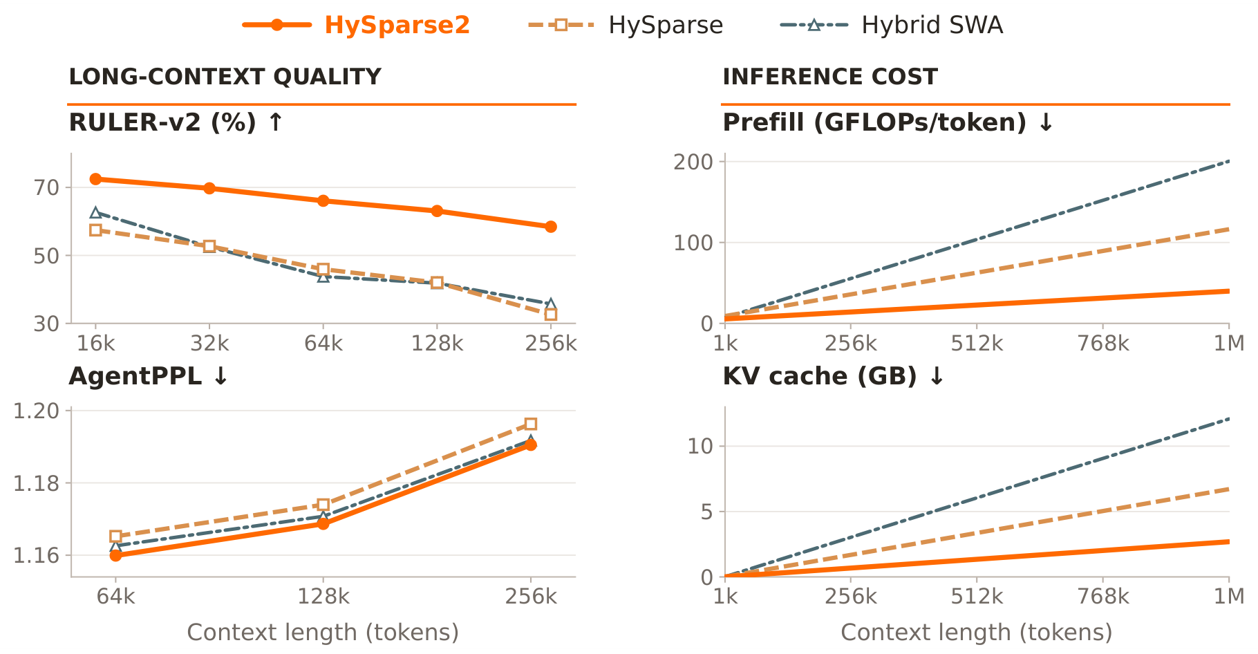
💡 Click any image for the full-resolution original (300 DPI); click again or press Esc to close.
Background: three demands
Section 2 of the paper lays out three threads of motivation, and every later design decision maps back onto one of them.
2.1 Efficient prefill: cheaper attention is not enough
Multi-turn agentic inference makes inference increasingly input-dominated — a single tool return can be orders of magnitude longer than the action that triggered it. The paper stresses one point: reducing attention cost alone does not remove the cost of propagating those tokens through the whole backbone. Even with a cheaper attention operator per layer, every layer's feed-forward still has to be computed.
Existing cross-layer KV sharing targets exactly this. YOCO (Sun et al., 2024) uses a self-decoder to build one global KV cache that the cross-decoder reuses, so prefill cache construction can exit after the self-decoder. Gemma 3n (Sanseviero and Ballantyne, 2025) adopts related cross-layer KV sharing to improve prefill efficiency. HySparse (Gao et al., 2026) does cross-layer sharing inside each hybrid sparse block: every full-attention layer hands its global KV cache and top-$k$ block indices to the sparse layers after it — but, as the paper points out, prefill still executes every layer.
2.2 The four axes of KV-cache compression
The paper sorts KV-cache compression into four axes. The taxonomy is worth keeping, because it fixes which cell this work occupies:
- Head: GQA/MQA let several query heads share KV heads (Ainslie et al., 2023; Shazeer, 2019), or MLA compresses KV into latent states (Liu et al., 2024a);
- Sequence: compress several tokens into fewer cache entries (DeepSeek-AI et al., 2026);
- Layer: share KV caches across layers (Brandon et al., 2024; Sun et al., 2024);
- Precision: lower the numerical precision of cached keys and values (Hooper et al., 2024; Liu et al., 2024b).
The paper's read is that prior work concentrates on intra-layer compression along the head, sequence, and precision axes, while HySparse2 pushes the layer axis — and not just at one level, but at two simultaneously: KV Bridging outside and KV Reuse inside.
2.3 Selection granularity: an inherent accuracy/efficiency trade-off
Sparse attention restricts each query to a subset of KV entries (Child et al., 2019), and the granularity of selection sets the accuracy/efficiency balance. HySparse originally chose block-level selection as a pragmatic compromise: evaluations showed no substantial accuracy disadvantage, and the regular block structure is friendly to efficient kernels.
But the paper argues that modern agentic workloads are long-horizon multi-turn trajectories that need precise retrieval from a long history. Under those patterns block-level selection shows a pronounced accuracy disadvantage, while token-level selection recovers relevant evidence more faithfully. At the same time, recent sparse-kernel progress (Wang et al., 2025) makes a token-level implementation practical. Together, those two facts justify the move from blocks to tokens.
Design rationale: three trade-offs
Section 3 reads as three trade-offs. Understanding them matters more than memorizing the architecture diagram, because the second one is the least replaceable step in the whole paper.
Trade-off 1: outer-level sharing happens only between full-attention layers
KV Bridging draws a hard boundary: it is established only between full-attention layers of the self-decoder and the cross-decoder — never touching SWA layers or sparse layers. The wording next to Eq. (1) reflects this, with $(i, j)$ being a full-attention-to-full-attention pair. The immediate benefit: the two decoders can use different hybrid ratios, so one self-decoder full-attention layer can supply several cross-decoder full-attention layers (in Figure 2 below, one supplies four).
Trade-off 2: remove the separate SWA branch and "force" the recent window into the selection
This is the paper's central argument and deserves restating in full. HySparse's sparse layers carry a separate gated SWA branch for local modeling. The paper observes that if such a branch were kept in the cross-decoder, the cross-decoder would have to project from its own hidden states to build a window-sized suffix of its KV cache — and those hidden states in turn depend on the hidden states of earlier layers. The paper calls this the cascading SWA dependency: the required token suffix grows linearly with depth, far longer than the window itself.
That leaves two options: compute those states during prefill (which means the cross-decoder cannot be skipped at all), or approximate them with something like bounded replay (DeepSeek-AI, 2026). HySparse2 takes a third route and removes the dependency by construction — the most recent 128 tokens are forced into the sparse selection set, so locality is served by reusing the same full-attention KV cache and needs no hidden states of its own. The paper notes this also removes the parameter cost of the separate projections in the gated baseline.
Trade-off 3: keep a few full-attention layers, and let them double as the indexer
Both HySparse2 and HySparse keep a small number of full-attention layers, for two reasons. First, full attention still matters for model quality. Second, those layers serve as the indexer, using exact attention scores to provide oracle token selection for the following sparse layers. That buys a clean training property: native end-to-end training with no separate indexer module and no auxiliary distillation objective to train one — in contrast to the routes that distil an indexer (Gao et al., 2024; DeepSeek-AI et al., 2025).
Full attention is expensive though, so its share is kept low. The paper offers two future directions: approximate the retained full-attention layers in post-training with a lightweight indexer plus sparse attention; or shift the compute allocation further toward sparsity — for instance reducing query heads in full-attention layers while increasing them in sparse-attention layers. The paper also states a deployment fact: in HySparse2, prefill KV-cache construction needs only one full-attention layer.
Method: what two-level KV sharing actually shares
HySparse2 keeps YOCO's backbone: the model is split into a self-decoder and a cross-decoder, and both use hybrid attention. What differs is the recipe — the self-decoder mixes full attention with sliding-window attention for local modeling, the cross-decoder mixes full attention with sparse attention for global retrieval. Sharing happens on two levels: KV Bridging across the two decoders outside, and KV Reuse inside each hybrid block. The figure below draws both at once:
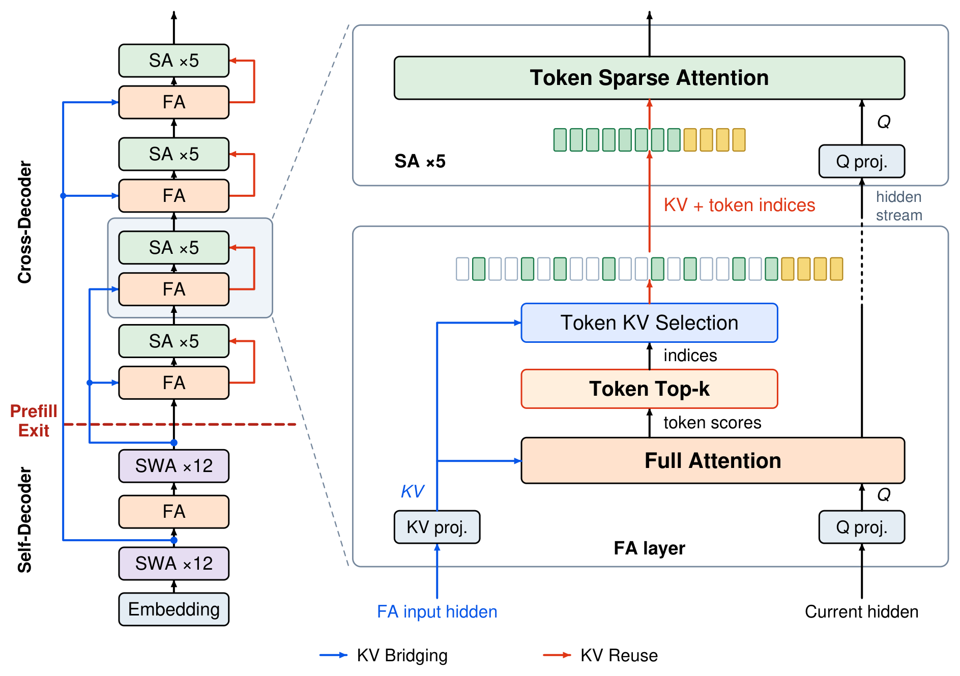
4.1 Outer level: KV Bridging
Take a pair of full-attention layers $(i, j)$, with $i$ in the self-decoder and $j$ in the cross-decoder. The paper defines the cross-decoder layer's K, V, and Q as:
Three things matter in that equation. First, the bridging source is $H_i^{\text{self}}$, the input hidden states of the self-decoder full-attention layer, not its output — the annotation in Figure 2 reads "FA input hidden" for exactly this reason. Second, K and V come from someone else's hidden states, but the projections are the layer's own: layer $j$ owns $\operatorname{Proj}_j^{K}$ and $\operatorname{Proj}_j^{V}$, so even when several layers share one hidden-state source, each still constructs a distinct KV cache. Third, Q still comes from the layer's own current hidden states, $\operatorname{Proj}_j^{Q}(H_j^{\text{cross}})$ — the attention still relates this layer's tokens to the shared history.
Together these three points make "one self-decoder full-attention layer supplies several cross-decoder full-attention layers" unambiguous: what is supplied is the source hidden states, not already-projected K/V, so each layer can still keep its own KV representation.
4.2 Inner level: two changes to KV Reuse
HySparse2 makes two modifications to HySparse's KV Reuse, both described in §3.3.
Change one: selection granularity moves from blocks to tokens
The mechanism is direct: apply top-$k$ selection to individual tokens in the full-attention layers, and let the following sparse layers reuse the KV entries of those selected tokens. The motivation comes from §2.3 — long-horizon multi-turn agentic tasks need more precise retrieval. The ablation in §4.3 tests this explicitly.
Change two: drop the separate SWA branch, force a local window instead
Inside a block, the selection set is assembled from two parts: a local window of the most recent tokens (always included), followed by the highest-scoring tokens outside that window. Both sets are read from the full-attention layer's KV cache and reused by the following sparse layers. The paper's configuration is 128 forced local tokens plus 1,024 global tokens (that is, $k_{\text{local}} = 128$ and $k_{\text{global}} = 1024$).
It is worth lining up how the three models handle locality: Hybrid SWA uses a 128-token sliding window; HySparse selects 1,024 global tokens in 64-token blocks plus a separate 128-token SWA branch merged by gated fusion; HySparse2 simply places 128 tokens into the selection set.
4.3 Mapping the configuration onto layer numbers [organized]
The paper never prints a layer table, but matching Figure 2's boxes against the stated 49 layers gives a reading that explains a lot:
- self-decoder = 25 layers: SWA×12 → FA → SWA×12, containing just one full-attention layer;
- cross-decoder = 24 layers: (FA + SA×5) repeated 4 times, i.e. 4 full-attention layers + 20 sparse layers;
- Total $25 + 24 = 49$ layers — 24 SWA, 20 SA, 5 FA — and the FA total of 5 matches Table 1's "#Full = 5".
Read together: the model has only 5 full-attention layers, and the single one in the self-decoder has to supply all four in the cross-decoder — that is what "different hybrid ratios, one-to-many bridging" looks like in the diagram; and of the 25 layers prefill must run, only one does full attention.
Inference system: disaggregation and speculative decoding
Section 3.5 translates the architectural property into a deployment plan. It is short but dense, and it decides what the design is actually worth in production.
5.1 Prefill–decode disaggregation: the prefill node hosts half a model
Under prefill–decode disaggregation, HySparse2's prefill node only has to host the self-decoder plus the KV Bridging projections. For the 49-layer model in Figure 2 that means deploying only the first 25 layers and cutting the prefill node's memory requirement by nearly half. And because the self-decoder's SWA-to-full-attention ratio is high, only 1 of those 25 layers does full attention.
One easily missed detail: the paper chooses to compute the cross-decoder's full-attention KV caches on the prefill node and transfer them to the decode nodes — because the projected KV caches are smaller than the source hidden states, so shipping KV beats shipping hidden states. That is a compute-for-bandwidth trade, and it also explains why KV Bridging uses per-layer projections rather than simply passing hidden states around.
5.2 Speculative decoding: an MTP layer now, a larger drafter later
During pretraining HySparse2 uses a single MTP layer conditioned on the hidden states at the self-decoder / cross-decoder boundary, to aid convergence. In post-training that layer could be replaced by a larger DFlash-style drafter (Chen et al., 2026) conditioned on the same boundary hidden states. The paper notes these hidden states become available early, which could support asynchronous drafting and verification (Zhang et al., 2025).
The paper is careful to hedge, though: training the larger drafter and coordinating asynchronous execution with verification feedback both remain future work. In other words §5.2 is a design-possibility argument, not a demonstrated result.
Experiments: setup, pretraining, post-training, cost
Evaluation has three parts — the overall comparison (model quality plus prefill FLOPs plus KV-cache size) and three ablations (sparse granularity, forced local window, KV Bridging). The organizing logic is clear: token-level selection buys long-context accuracy, the forced window and KV Bridging buy prefill cost, and quality is required not to move.
6.1 Setup: three models differing only in attention design
Unless stated otherwise the experiments use 80B-A3B MoE models: 49 Transformer layers, hidden size 2,048, and a simplified mHC variant (Xie et al., 2026; Zhu et al., 2025). The only difference between the three models is the attention design:
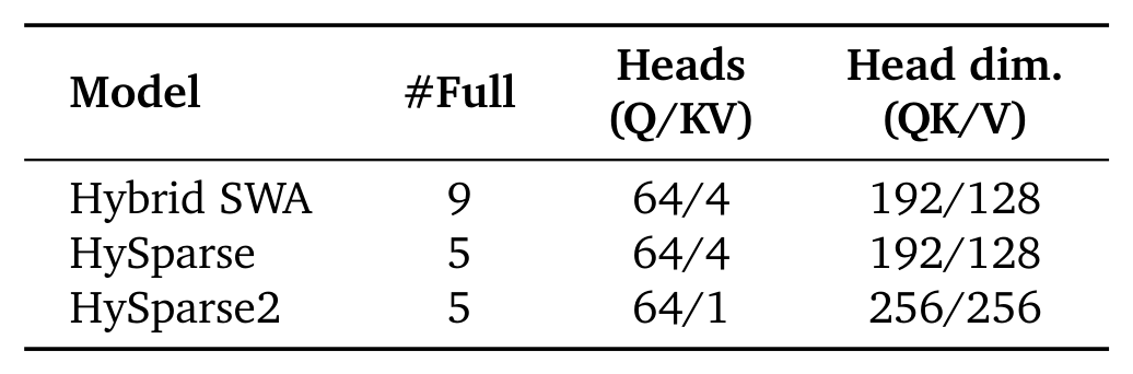
A few more configuration details are worth recording. Within HySparse2's self-decoder, the SWA layers use partial RoPE (64 rotary dimensions, base 10,000) while the full and sparse attention layers use NoPE — which is why the paper stresses that HySparse2 needs no RoPE adjustment for long-context extension. Across all three configurations, every sparse and SWA layer uses sigmoid output gates (Qiu et al., 2025) and learnable per-head sink biases (Agarwal et al., 2025).
On training: pretraining runs about 500B tokens at a 32k context; a light post-training stage adds roughly 100B tokens, introduces agentic data into the mixture, and extends the context to 256k. Within each stage all three models share the same data mixture and schedule. The Muon optimizer (Jordan et al., 2024) with a WSD schedule, peak learning rates $10^{-3}$ for pretraining and $5\times10^{-5}$ for post-training. The overall comparison reports both pretraining and post-training results; ablations report pretraining only.
Evaluation spans four families: knowledge (MMLU, MMLU-Redux, C-Eval, CMMLU, TriviaQA), reasoning (BBH, MATH, DROP, GSM8K, ARC-C, HellaSwag, WinoGrande), code (HumanEval+, MBPP+, Repo Code PPL) and long context (RULER, NoLiMa). Repo Code PPL is an internal benchmark reporting byte perplexity over long code repositories with cross-file dependencies, so it also probes long-context modeling. The post-training stage focuses on two groups: multi-turn retrieval (MRCR-v2, RULER-v2, GraphWalks) and long-context likelihood (AgentPPL, LongPPL). AgentPPL is an internal benchmark built from multi-turn agent trajectories, reporting byte perplexity on the reasoning, tool-call, and response segments of 1,000 trajectories; LongPPL (Fang et al., 2024) computes perplexity only on selected tokens that depend on long-range context, over 349 examples; MRCR-v2 (Vodrahalli et al., 2024) is multi-round retrieval with 2/4/8 needles; RULER-v2 (Hsieh et al., 2025) covers 12 retrieval and QA subtasks; GraphWalks (OpenAI, 2025) tests multi-hop graph traversal. Retrieval averages weight the reported context lengths equally.
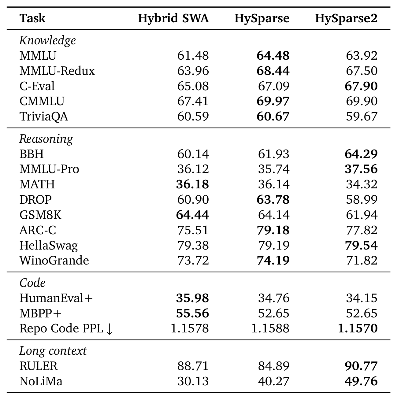
6.2 Pretraining: strongest on long context, a mixed account elsewhere
6.3 Post-training: ahead on four metrics at every length
After the same light post-training stage of about 100B tokens, the picture gets much cleaner:
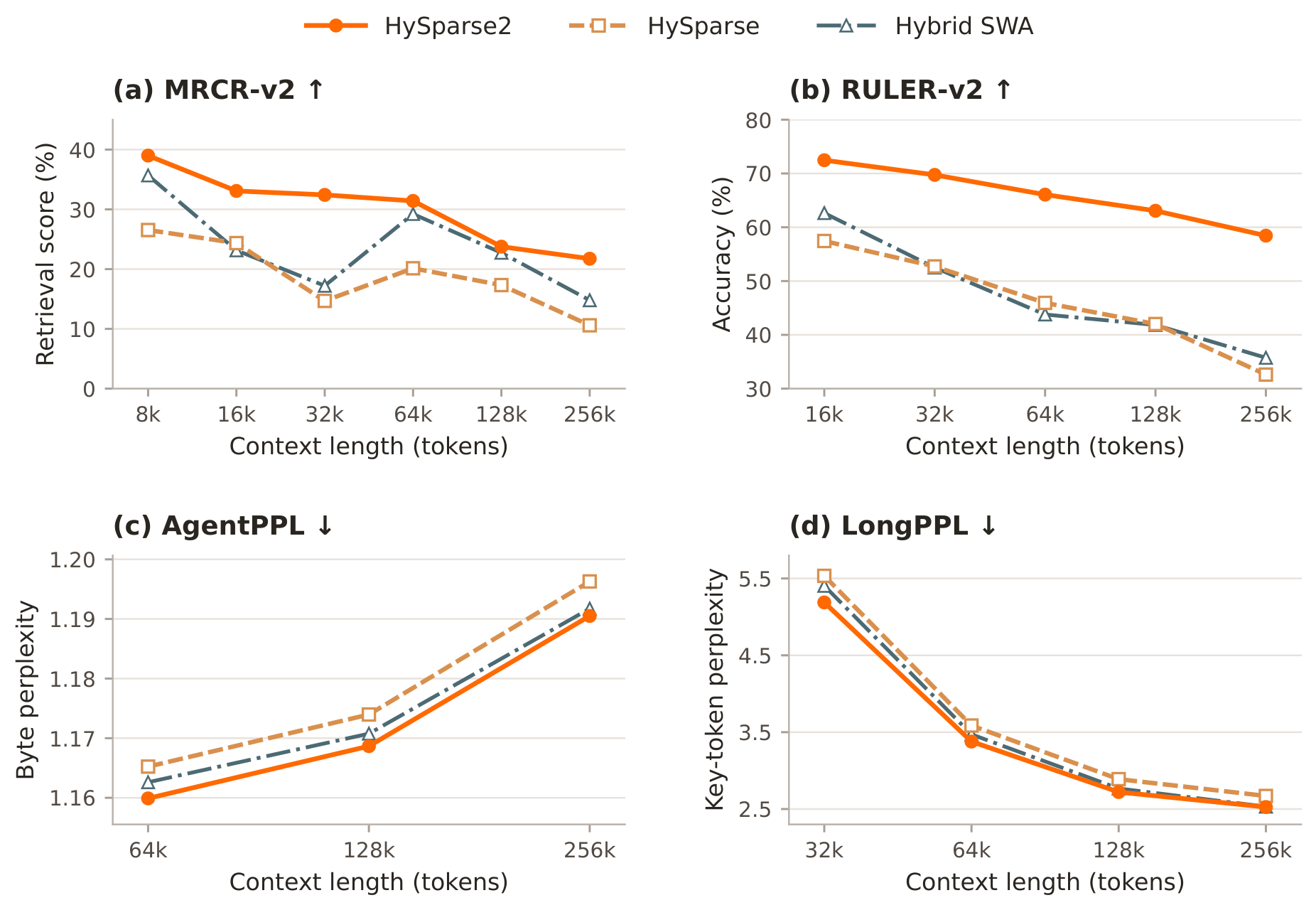
The paper's headline averages: relative to HySparse, mean MRCR-v2 +11.30 and RULER-v2 +19.81 points; relative to Hybrid SWA, +6.44 and +18.65. HySparse2 also achieves lower AgentPPL and LongPPL across the whole evaluated range, so the retrieval gains come together with better likelihood on long agent trajectories and on context-dependent tokens.
6.4 Cost: prefill FLOPs and KV cache
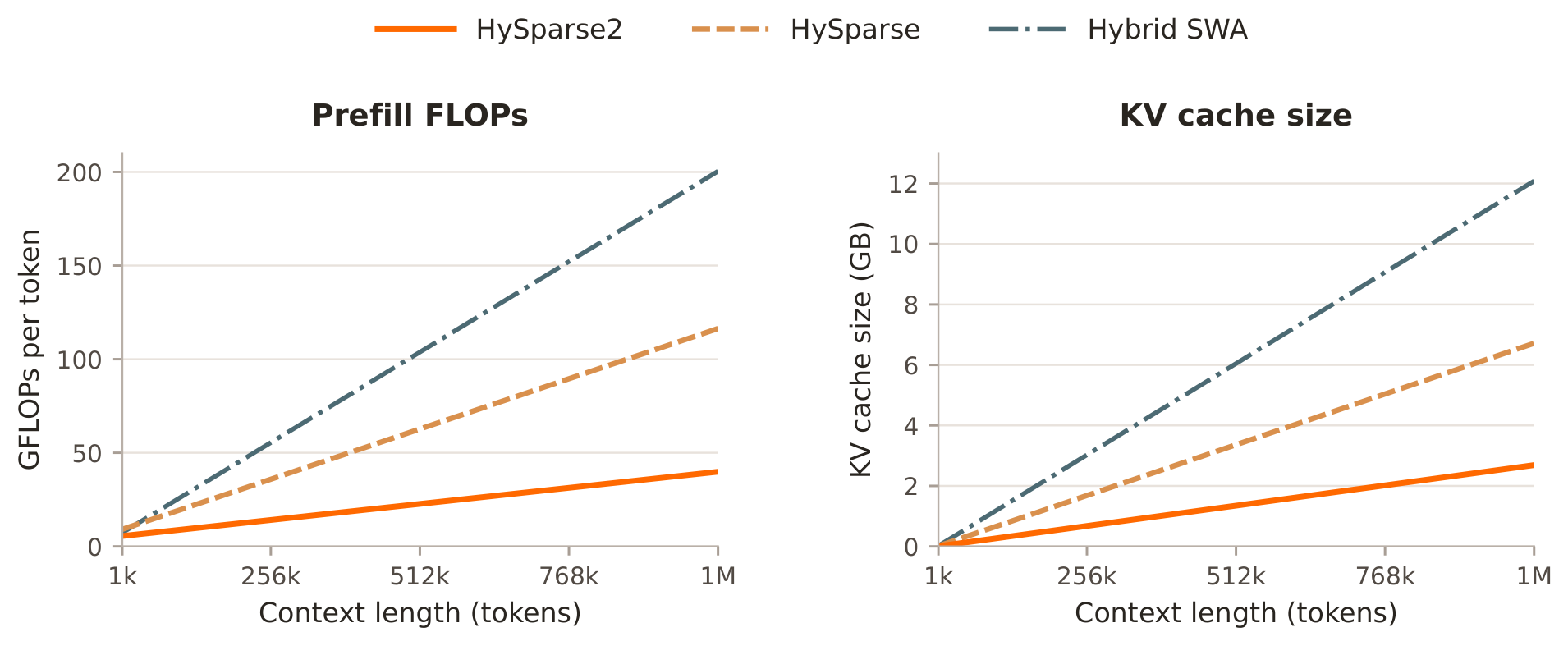
The KV-cache account, item by item [estimated]
The paper gives three totals and no breakdown. But Table 1's KV-head configuration is enough to re-derive them, and the result happens to confirm an important design claim:
- KV bytes per token per layer = KV heads × (head dim K + head dim V) × 1 byte (FP8);
- HySparse2 (MQA 64/1, head dim 256/256): $1 \times (256+256) = 512$ bytes per layer per token; with 5 FA layers → 2,560 bytes/token;
- HySparse (GQA 64/4, head dim 192/128): $4 \times (192+128) = 1{,}280$ bytes per layer per token; 5 FA layers → 6,400 bytes/token;
- Hybrid SWA (same GQA configuration): 1,280 bytes per layer per token; 9 FA layers → 11,520 bytes/token.
Multiplying by 1M tokens gives 2.56 / 6.40 / 11.52 GB against the paper's 2.69 / 6.72 / 12.09 GB.
None of the three matches exactly, but all three are off by the same factor (about 1.05×) — which points to a uniform unit or bookkeeping convention rather than a structural difference. What actually carries information is the pairwise ratios: the derived $6{,}400/2{,}560 = 2.50$ and $11{,}520/2{,}560 = 4.50$ line up almost exactly with $6.72/2.69 = 2.50$ and $12.09/2.69 = 4.49$ computed from the paper's numbers.
That confirms two things. First, the three models' cache sizes are essentially determined by "FA-layer count × KV-head configuration". Second, the sparse layers carry no resident KV cache at all — they really do read the block's full-attention cache, which is exactly the accounting effect KV Reuse is supposed to produce. It also makes clear that part of HySparse2's 2.50× advantage over HySparse comes from the MQA change rather than from cross-layer sharing alone: if KV heads were held at GQA 64/4, the FA-layer count difference on its own would explain only $9/5 = 1.8\times$.
Ablations: three questions, three controls
The three ablations correspond to three design decisions, and all report pretraining results only (within the 32k training context). That matters for interpretation — especially for the first one, whose motivation is a 256k agentic scenario.
7.1 Granularity: token-level vs block-level, same budget
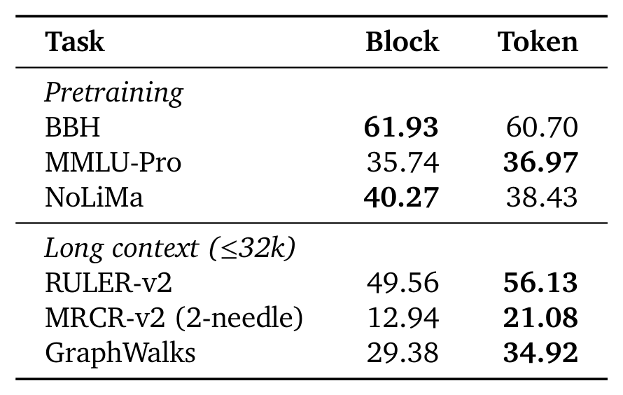
The paper's explanation of the gain deserves quoting in its own right: agent trajectories repeatedly interleave reasoning, tool calls, and returned observations, and the information needed for an answer may be spread across several turns together with role delimiters and other special tokens (those are what mark the relevant boundaries). Under a fixed budget, selecting a whole block in order to keep one such token also spends capacity on its neighbours; token-level selection can allocate that budget to individual positions across the context. The retrieval and graph-reasoning gains are consistent with that account.
7.2 Local window: forced membership vs a separate branch
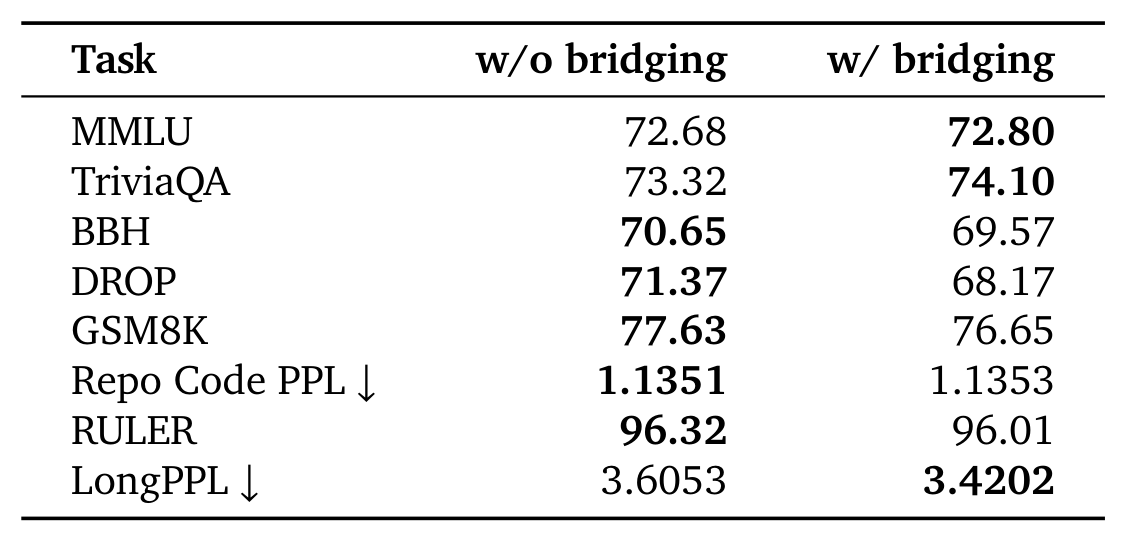
7.3 KV Bridging: is the prefill gain free?
The key question is whether KV Bridging — designed mainly to accelerate prefill — costs quality. The paper tests it in two directions.
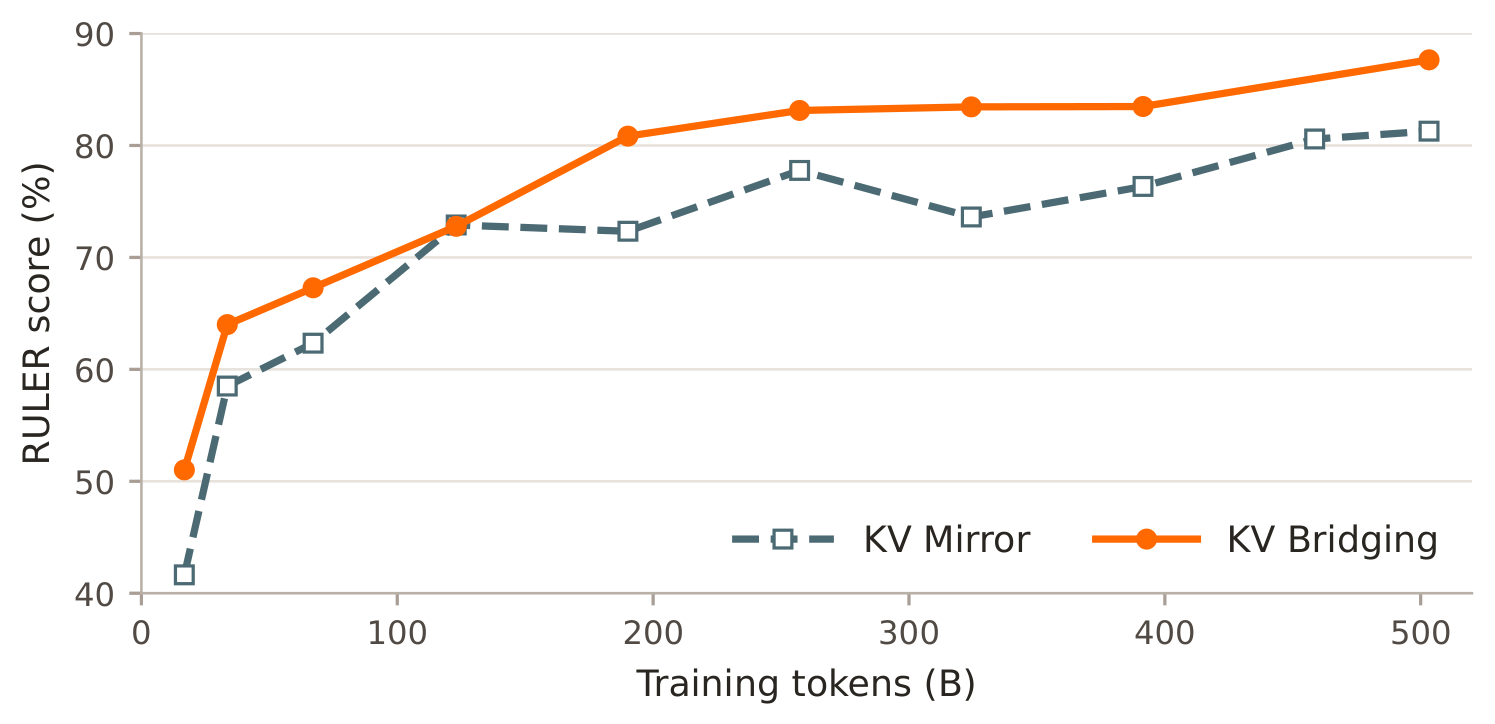
The second direction is the connection scheme itself. The paper compares KV Bridging against KV Mirror (Liu et al., 2026) on the same hybrid backbone and pretraining recipe:
Commentary: strengths, limits, and the accounts to watch
Strengths
- The argument is closed, not a pile of tricks. The paper does not stop at "we saved FLOPs"; it completes the causal chain: separate SWA branch → depends on cross-decoder's own hidden states → cascading dependency makes the token suffix grow with depth → the cross-decoder cannot be skipped → therefore locality must be rewritten as fixed membership in the selection set. That ordering makes "prefill runs half the model" a derivable conclusion rather than an assertion.
- The ablation controls are clean. §7.1 holds backbone, 1,024-token global budget, and 128-token local window fixed and moves only the selection unit; §7.2 shares backbone, KV Bridging and self-decoder and moves only how the cross-decoder handles locality. One-variable-at-a-time controls like these are not that common.
- The key mechanism is re-verified at larger scale. The KV Bridging ablation is run at 290B-A8B / ~1.8T tokens rather than only at 80B — a step architecture papers often skip.
- Honest about its reference baselines. The paper states plainly that full attention in every layer is the strongest reference, that Hybrid SWA needs 9 full-attention layers because fewer significantly degrades accuracy, and that HySparse2 trails HySparse on DROP. Reversals are not hidden.
- Architectural constraints are expressed in deployment terms. The prefill node hosts 25 layers; KV rather than hidden states is transferred because it is smaller — design decisions map directly onto deployment decisions, so a reader can price them.
- It leaves a testable next step. Reduce query heads in FA layers and increase them in SA layers to push compute further toward sparsity — a concrete, falsifiable direction.
Limits and accounts to watch
- What "broadly comparable" actually contains. In Table 2 HySparse2 is 4.79 points below HySparse on DROP, 2.20 on GSM8K, 1.82 on MATH and 2.37 on WinoGrande; against Hybrid SWA it is 2.91 below on MBPP+ and 1.91 on DROP. The general-capability cost lands mainly on reasoning and code tasks and is summarized in one sentence as "a mixed picture".
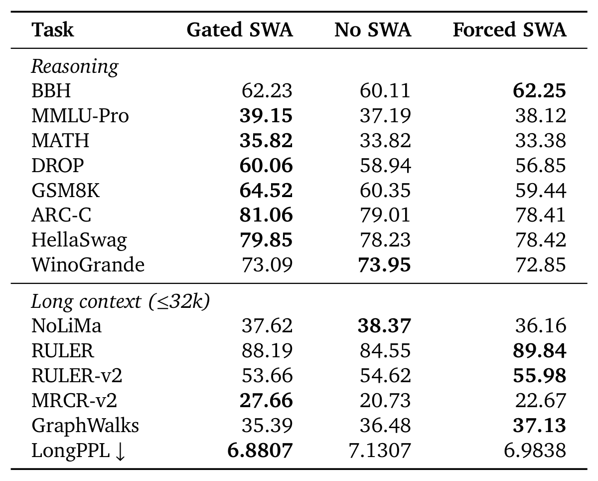
- The accuracy cost concentrates in the metrics it champions. §7.2 shows Forced SWA 4.99 points below Gated SWA on MRCR-v2, 5.08 below on GSM8K, and 1.50% worse on LongPPL. MRCR-v2 is one of the two retrieval metrics used to argue retrieval is stronger, and GSM8K is a reasoning task. The paper calls the trade acceptable on the grounds that it swaps parameters and a local KV cache for early-exit capability — but the reader should judge the bargain.
- Reversals in the granularity ablation go unmentioned. In Table 3, NoLiMa (40.27 vs 38.43) and BBH (61.93 vs 60.70) both favour block-level. The prose does not raise either.
- The KV-cache advantage is partly the head configuration's doing. HySparse2 uses MQA 64/1 while both baselines use GQA 64/4 (Table 1), so the size advantage in §6.4 is not purely cross-layer sharing. The paper provides no MQA-vs-MQA or GQA-vs-GQA control to separate the two. By this page's estimate, ignoring the head difference, "5 FA layers against 9" would explain only $9/5 = 1.8\times$ rather than the observed 4.49×.
- Ablation context length does not match the motivation. §7.1 is motivated by long-horizon multi-turn agentic retrieval, yet the ablation runs inside the 32k training context — the paper itself notes "These gains are present within the 32k training context". The same control at 256k remains to be run.
- All costs are book figures. Every cost conclusion rests on FLOPs and KV-cache bytes with no end-to-end throughput or latency measurement; the claimed token-level kernel efficiency advantage is likewise unmeasured. §5.2's speculative-decoding part is a possibility argument the paper itself flags as future work.
- Some metrics are not comparable across papers. AgentPPL and Repo Code PPL are internal benchmarks; LongPPL's selection over 349 examples and MRCR-v2's needle combinations are described only coarsely. These numbers are valid within this paper's internal comparisons but should not be lined up against other papers' nominally similar metrics.
Lineage at a glance
This page reorganizes the technical sources cited in the paper by component, to make clear what is new here and what is inherited and modified.
| Component / decision | Upstream as cited by the paper | What this generation changed |
|---|---|---|
| Two-decoder backbone + early-exit prefill | YOCO (Sun et al., 2024); related cross-layer sharing in Gemma 3n (Sanseviero and Ballantyne, 2025) | KV Bridging connects only full-attention layers, allowing different hybrid ratios in the two decoders — one self-decoder FA layer supplies four cross-decoder FA layers |
| Cross-layer KV / index sharing inside a hybrid block | HySparse (Gao et al., 2026) | Kept as the inner-level KV Reuse; the selection unit moves from 64-token blocks to individual tokens |
| Oracle selection with no separate indexer | HySparse (Gao et al., 2026); contrasting routes: SeerAttention (Gao et al., 2024), DeepSeek-AI et al. (2025) | Top-$k$ over single tokens; no distilled auxiliary indexer needed, native end-to-end training |
| Handling locality | HySparse's separate gated SWA branch (Gao et al., 2026) | Branch deleted; the most recent 128 tokens are forced into the sparse selection, and locality comes from the shared KV cache |
| Rejected alternative | bounded replay (DeepSeek-AI, 2026) | Rather than approximating, the dependency on cross-decoder hidden states is removed by construction |
| Feasibility of token-level sparse kernels | TileLang (Wang et al., 2025) | Used to argue token-level selection is now practical to implement |
| KV head configuration | MQA (Shazeer, 2019); GQA (Ainslie et al., 2023) | Switched to MQA 64/1 (baselines use GQA 64/4) for a smaller KV cache and better token-sparse kernel efficiency |
| Positional encoding | RoFormer / partial RoPE (Su et al., 2024); NoPE | SWA layers use 64-dim partial RoPE (base 10,000); full and sparse layers use NoPE — no RoPE adjustment needed for long-context extension |
| Attention post-processing | Sigmoid output gates (Qiu et al., 2025); per-head sink bias (Agarwal et al., 2025) | Applied uniformly to all sparse and SWA layers |
| Backbone and residuals | mHC (Xie et al., 2026; Zhu et al., 2025) | Simplified variant with the residual mixing matrix fixed to the identity |
| Optimizer and schedule | Muon (Jordan et al., 2024) | WSD schedule; peak LR $10^{-3}$ (pretraining) / $5\times10^{-5}$ (post-training) |
| Connection-scheme control | KV Mirror's U-shaped pairing (Liu et al., 2026) | Changed to full-attention layers only; reported final RULER 87.65 vs 81.28 |
| Speculative decoding / MTP | DFlash (Chen et al., 2026); asynchronous drafting and verification (Zhang et al., 2025) | MTP layer conditioned on the self/cross boundary hidden states; a larger drafter is future work |
| Long-context likelihood metric | LongPPL (Fang et al., 2024) | Adopted as-is; AgentPPL is this paper's internal benchmark |
| Evaluation suites | MRCR (Vodrahalli et al., 2024); RULER-v2 (Hsieh et al., 2025); GraphWalks (OpenAI, 2025); NoLiMa (Modarressi et al., 2025) | — |
Citations follow the paper's own inline attributions; this page has not re-checked each reference entry.
Not disclosed, worth testing next
- The token-score algorithm. The paper says full-attention layers use "exact attention scores" to give the following sparse layers oracle selection, and Figure 2 only labels "token scores" and "Token Top-k". But how scores are aggregated across query positions and across query heads into one score per KV token (which statistic, whether only particular queries count, whether any extra normalization is applied) is not disclosed — and this determines the indexer's cost and is the first obstacle to reproduction.
- End-to-end throughput and latency. The paper reports only FLOPs and KV-cache bytes (a full-text search turns up no mention of throughput, latency, or TTFT). A measurement of real-kernel prefill latency and decode throughput is worth adding, especially at 1M context under the disaggregated deployment where the prefill node hosts 25 layers.
- Prefill → decode KV transfer cost. The paper computes the cross-decoder FA KV on the prefill node and ships it to decode nodes because "the projected KV caches are smaller than the source hidden states". The transfer volume, the benefit under a bandwidth constraint, and the combined benefit with "the prefill node hosts 25 layers" are not quantified.
- Sensitivity of the forced window. The window is fixed at 128 and the global budget at 1,024, with no sensitivity sweep. Given that Forced SWA is 4.99 points below Gated SWA on MRCR-v2, it is worth trying a longer window, or a gated variant inside the window, to see whether that gap can be recovered.
- Granularity ablation at 256k. The token-vs-block control was run within the 32k training context while its motivation is 256k multi-turn agentic retrieval. Repeating it at long context — and reproducing the Table 3 reversals on NoLiMa and BBH — is the key step in judging whether token-level is generally better.
- Separating head configuration from cross-layer sharing. A control with both models on MQA (or both on GQA) would split the KV-cache and kernel-efficiency gains into "cross-layer sharing" and "number of KV heads".
Glossary
Come back here whenever an abbreviation appears; underlined abbreviations in the prose also carry hover definitions.
| Abbrev. / term | Full name | One-line explanation |
|---|---|---|
| FA | Full Attention | Every query sees the entire history; most accurate, most expensive — only 5 layers here |
| SWA | Sliding-Window Attention | Attends only to a recent fixed window; handles local modeling — 24 layers in the self-decoder |
| SA | Sparse Attention | Each query attends only to a selected subset of KV entries — 20 layers in the cross-decoder |
| KV Bridging | — | This paper's outer-level sharing: a cross-decoder FA layer projects its own K/V from the input hidden states of a self-decoder FA layer |
| KV Reuse | — | This paper's inner-level sharing: within a hybrid block, SA layers reuse the FA layer's KV cache and selection indices |
| KV Mirror | — | The comparison connection scheme: reverse U-shaped pairing of early and late layers ($1 \rightarrow n$, $2 \rightarrow n-1$); its RULER trails KV Bridging in Figure 5 |
| hybrid block | — | Here, a group like "FA + SA×5"; the cross-decoder is made of four such groups |
| cascading SWA dependency | — | A separate SWA branch needs its own hidden-state suffix, which itself depends on earlier layers, so the required length grows linearly with depth — the root reason the cross-decoder cannot be skipped |
| block-level / token-level | — | Sparse selection granularity: 64-token blocks versus single tokens. This paper moves from the former to the latter |
| forced local window | — | The most recent 128 tokens are always included in the sparse selection set, replacing the separate SWA branch |
| indexer | — | A module predicting which KV entries are worth selecting. Here the FA layers serve as the indexer, so none is trained separately |
| oracle token selection | — | Selection signal derived from exact attention scores rather than an approximation module |
| gated fusion | — | How HySparse merges sparse attention with a separate SWA branch under a gate; HySparse2 removes this structure |
| sink bias | — | A learnable per-head bias that mitigates the attention-sink phenomenon |
| YOCO | You Only Cache Once | An architecture where a self-decoder builds one global KV cache reused by the cross-decoder, letting prefill exit after the self-decoder |
| MQA / GQA / MLA | Multi-Query / Grouped-Query / Multi-head Latent Attention | Three head-axis KV compression schemes: one shared KV set for all query heads / grouped sharing / compressed into latent states. HySparse2 uses MQA 64/1 |
| RoPE / NoPE | Rotary / No Positional Embedding | Rotary position encoding / no explicit positional encoding. Here only SWA uses 64-dim partial RoPE |
| MoE | Mixture-of-Experts | 80B-A3B means 80B total parameters with roughly 3B activated per token |
| mHC | Manifold-constrained Hyper-Connections | A residual-connection variant; the simplified form here fixes the residual mixing matrix to the identity |
| MTP | Multi-Token Prediction | An extra prediction layer usable as a speculative drafter; conditioned on the self/cross boundary hidden states here |
| Prefill / Decode | — | The two inference stages: one forward pass over the input to build the KV cache / autoregressive generation token by token |
| Prefill–Decode Disaggregation | — | Serving the two stages on separate nodes, each tuned to its own profile; the prefill node here hosts only 25 layers |
| FP8 | 8-bit Floating Point | The precision basis for this paper's KV-cache figures (1 byte per element) |
| GFLOPs / token | — | Billions of floating-point operations per token, the measure of prefill compute |
| PPL | Perplexity | Lower is better; AgentPPL / LongPPL / Repo Code PPL are three different variants |
| AgentPPL | — | This paper's internal benchmark: byte perplexity on the reasoning, tool-call and response segments of 1,000 multi-turn agent trajectories |
| LongPPL | — | Perplexity computed only on selected tokens that depend on long-range context (Fang et al., 2024); 349 examples here |
| needle | — | A fact planted inside a long document in retrieval evaluation; MRCR-v2 uses multi-round 2/4/8-needle settings |
| RULER / RULER-v2 | — | Long-context benchmarks; v2 covers 12 retrieval and QA subtasks |
| MRCR-v2 | — | Multi-round retrieval benchmark (following the MRCR line of Vodrahalli et al., 2024) |
| GraphWalks | — | Multi-hop graph traversal evaluation (OpenAI, 2025), probing reasoning-style retrieval across passages |
| bounded replay | — | A method that approximates required hidden states by replaying a bounded length; this paper avoids needing it by construction |